This series examines the Federal Reserve Bank of New York’s dynamic stochastic general equilibrium (FRBNY DSGE) model—a structural model used by Bank researchers to understand the workings of the U.S. economy and provide economic forecasts.
The severe recession experienced by the U.S. economy between December 2007 and June 2009 has given way to a disappointing recovery. It took three and a half years for GDP to return to its pre-recession peak, and by most accounts this broad measure of economic activity remains below trend today. What precipitated the U.S. economy into the worst recession since the Great Depression? And what headwinds are holding back the recovery? Are these headwinds permanent, calling for a revision of our assessment of the economy’s speed limit? Or are they transitory, although very long-lasting, as the historical record on the persistent damages inflicted by financial crisis seems to suggest? In this post, we address these questions through the lens of the FRBNY DSGE model.
DSGE models are a particularly suitable tool to look under the economy’s hood and illuminate its inner workings. Their structure allows us to decompose the evolution of the key macroeconomic variables that we can measure—such as GDP and inflation—in terms of their underlying driving forces, which are unobserved. In terms of the automotive metaphor, with a model of the car/economy in hand, we can trace back its observed behavior—direction and speed, say—to its fundamental determinants, such as the conditions of the road and the actions of the driver on the accelerator and the brakes. The key difference of course is that the economy is much more complicated than a car, and does not have one driver behind the wheel. Therefore our model can only provide a simplified, and in many cases imperfect, account of its workings. Even with these simplifications, however, the model provides useful insights.
The FRBNY DSGE model attributes the observed movements in macroeconomic variables to several fundamental disturbances, as explained in the previous post in this series and in more detail in our staff report. As it turns out, only four of these shocks account for the bulk of the movements in GDP and inflation since the Great Recession.
- A shock to total factor productivity (TFP), which affects the overall ability of the economy to produce output from any given amount of labor and capital inputs. A positive TFP shock results in higher GDP and, at the same time, in lower costs of production and hence lower inflation. In our model, shifts in TFP have a permanent effect on the economy’s productive potential. They capture a whole range of “structural” factors that will affect the growth trajectory of the economy for the foreseeable future.
- A financial (or spread) shock stemming from increases in the perceived riskiness of borrowers, which induces banks and other intermediaries to charge higher interest rates on loans, thereby widening credit spreads. An increase in perceived risk (a positive realization of this shock) leads to a large increase in the cost of capital for entrepreneurs, which depresses investment demand and hence GDP growth. As a result of the lower demand, inflation also falls. Although the spikes in spreads associated with this shock tend to be relatively short-lived, as they were during the crisis, their effects can linger well past the most acute phase of market disruptions, with persistently tight credit conditions depressing demand, and hence output and inflation, for several years. Unlike the TFP shocks, however, these financial disturbances are not permanent, and their effects will ultimately dissipate, returning the economy to its pre-crisis growth trajectory.
- A shock to investment demand, whose negative realizations persistently depress capital formation, leading to lower growth and lower inflation. This shock has very similar macroeconomic effects to the risk shock we just described, with the crucial difference that it does not move credit spreads. Therefore, this disturbance can be thought of as capturing financial and other factors that do not manifest themselves in higher spreads, but that nonetheless affect firms’ willingness or ability to invest. Examples of such factors are a reluctance to lend by banks that does not lead to higher interest rates on loans, but for instance to a rationing of credit to certain borrowers, as well as the perception by firms of a particularly uncertain outlook, which delays their investment decisions.
- Shocks to monetary policy, capturing changes in the monetary policy stance not reflected in the policy rate, such as the introduction of forward guidance.
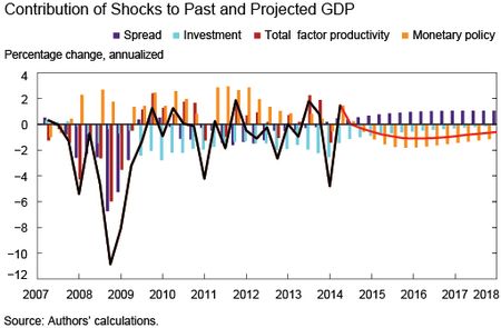
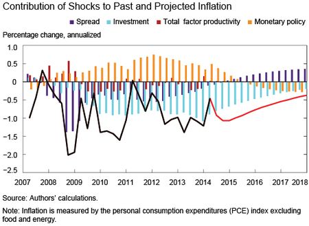
The two charts below present the contributions of these four factors to the evolution of past observed and future projected GDP growth and inflation between 2007 and 2018. The variables are in deviation from their sample mean. Released data are represented by the black line. The projections for the rest of 2014 and beyond, captured by the red line, come from the model, as explained in more detail in the last post in this series. The colored bars represent the contribution of the corresponding driving force to the observed (or projected) outcome at any given point in time.
The first feature of this decomposition that we want to highlight is the paramount importance of spread shocks (in purple) during the recession. Starting at the end of 2007, the economy experiences a sequence of large shocks to credit spreads, driven by an increase in the perceived riskiness of borrowers. This progressive increase in risk is accompanied by deteriorating credit conditions, culminating in two spikes in spreads in the third and fourth quarters of 2008 with the failure of Lehman Brothers. These abrupt increases in the cost of credit account for a decline in quarterly GDP growth of more than 5 percentage points (annualized), which is about half of the total drop in output growth at the nadir of the recession. Inflation is also significantly affected by these shocks, which account for about three quarters of the decline in inflation in the second half of 2008.
The other half of the decline in GDP growth in 2008 stems from significant declines in TFP (the red bars). As we already pointed out, TFP shocks have permanent effects on the productive capacity of the economy in our framework, suggesting that the recession caused some lasting damage. However, the negative shocks of 2008 are followed by positive shocks, with the red bars primarily contributing to GDP growth. As a result, the level of TFP, and hence of potential output in our model, emerges largely unscathed at the present time.
As 2008 unfolds and the recession quickly worsens, the only force pushing against the fast deterioration in economic conditions is monetary policy. The orange bars—monetary policy shocks—do not represent the overall reaction of monetary policy to economic developments, which includes changes in the policy rate, but rather the extent to which this reaction exceeds what “normal,” historical reaction patterns would imply. Therefore, the large contributions of the orange bars suggest that the Federal Reserve was particularly aggressive in fighting the crisis early on, deploying several tools that went beyond its conventional weaponry. According to our model’s accounting, this extra effort is worth 2 to 3 percentage points of annual GDP growth in the middle of 2008, for a total boost to GDP of roughly 2 percent for 2008 as a whole. And this estimate does not even include the effects of the many credit and liquidity programs the Fed engaged in to ameliorate conditions in financial markets at the height of their stress.
Moving on to the recovery phase, which according to NBER dating starts in the middle of 2009, we can see that shocks to investment demand (in light blue) are the main headwinds holding back the economy. As credit spreads return to normal, the effect of financial risk shocks (in purple) dissipates, even though their overall effect continues to be a drag on growth and inflation. At this point, however, investment shocks start taking on a very large negative role in pushing down both GDP growth and inflation. The key feature of these shocks is the persistence of their effect on both variables, which remain depressed throughout the recovery phase, and into the forecast horizon. Admittedly, the fundamentals of investment shocks are harder to characterize than those of the spread or TFP shocks, representing any factor unrelated to credit spreads that might still restrain investment demand. Many such factors have been identified over time as playing a role in the sluggish recovery, including an overall reluctance of banks and other intermediaries to expose their balance sheets to risk, regardless of the pricing of that risk, and the tendency of firms to delay projects in the face of unusually uncertain prospects. Either way, our model squarely points to investment demand shocks as playing a fundamental role in retarding the recovery, consistent with the view that weak investment, more than consumption, has been behind the slow pace of growth and subdued inflation.
Monetary policy remains on the other side of the ledger over the recovery period, serving to counteract the negative effects of the shocks weighing on the economy. Even with the policy rate against its zero lower bound, monetary policy continues to lift economic activity and prevent inflation from falling too far below target, as demonstrated by the positive orange bars in the chart. In the model, this stimulus is achieved through forward guidance, whose effect on expected future policy rates, and hence on long-term rates, is explicitly taken into account in the model estimation.
The model’s forecast for the evolution of the economy over the next few years (the red lines in both charts) remains persistently subpar, with GDP growth about half a percentage point below its mean and inflation recovering very slowly—scenarios that will be discussed in more detail in the last post in this series. Decomposing the forecasts into their determinants highlights two main features. First, the headwinds represented by tight credit and the other factors holding back investment demand abate only gradually, contributing to restrain the economy over the medium term. Second, monetary policy starts representing a drag on growth and inflation over the forecast horizon, even though the policy rate remains lower than it would otherwise be. The reason is that, in the model, monetary policy has no long-run effects on the real economy, so monetary policy shocks can only affect the level of output temporarily.
In conclusion, this analysis finds little evidence of the permanent structural damage to the economy’s productive potential that many commentators see as the main culprit for the subpar recovery from the Great Recession. Instead, our decomposition is quite supportive of the narrative popularized by Reinhart and Rogoff and more recently by Mian and Sufi, according to which a slow recovery is what we should have expected owing to the very persistent damage inflicted by the financial crisis on the real economy. In the FRBNY DSGE model, this damage manifests itself as a sequence of negative shocks to investment demand—shocks that capture many of the headwinds often mentioned as an impediment to a more robust recovery. At the same time, our model suggests that monetary policy played an important role in cushioning the blow from the financial crisis and in sustaining the recovery, which could have been significantly more disappointing without the aggressive actions undertaken by the Fed.
Disclaimer
The views expressed in this post are those of the authors and do not necessarily reflect the position of the Federal Reserve Bank of New York or the Federal Reserve System. Any errors or omissions are the responsibility of the authors.
Andrea Tambalotti is an officer in the Federal Reserve Bank of New York’s Research and Statistics Group.
Argia M. Sbordone is a vice president in the Bank’s Research and Statistics Group.


 RSS Feed
 Follow Liberty Street Economics
Charles and Michael, you are right, enriching the model with a more granular description of investment, allowing for separate residential and equipment expenditures, for instance, or with a banking sector subject to capital requirements, would allow the model to address even more questions than the ones we are tackling in this post. As explained in our post on Tuesday, DSGE modelers have a tendency to err on the side of parsimony, so as to focus on the specific questions they are most interested in. That was the choice we made in this case. However, other DSGE models do include some of the features you are pointing out, so we can gain some insights on the questions you raise from looking at those models. As for the “milk spill” mentioned by pwinghart (i.e. the boom in housing and commodities around 2006), there is a debate among economists on its ultimate causes and it would certainly be interesting to study what our model has to say about that. An excellent idea for a future blog entry! Finally, on TFP, which is mentioned by both pwinghart and Brian, it is true that, to a certain extent, it is a “back-solved” plug, like all the shocks in DSGE models are. In fact, this a colorful, but pretty accurate description of how the Kalman filter “solves” for the paths of shocks that make the model consistent with the observable variables, as we explained in Tuesday’s post. Yet, independent measures of TFP based on entirely different methodologies, such as that developed by the San Francisco Fed and published quarterly here (http://www.frbsf.org/economic-research/total-factor-productivity-tfp/), tell a remarkably similar story, providing some reassurance that those “plugs” do indeed hold some water…
I think it is great that you guys are providing some insights into your DSGE model. The one question this post raises is whether the model is overwhelmed by unmodeled factors. You write: “The other half of the decline in GDP growth in 2008 stems from significant declines in TFP (the red bars)” and that the TFP factor “capture[s] a whole range of “structural” factors that will affect the growth trajectory of the economy for the foreseeable future.” How are we to read this as anything other than a back-solved “plug” where the unexplained factor is highly significant. Also, without further exposition, it is difficult to assume that there is some, sudden unobserved change in TFP that occurred just at the onset of the crisis.
Excellent analysis although I’m disappointed in the absence of the yet unsolved “conundrum” of 2005, especially the clear impact it had in the housing and commodity markets starting as early as 2006. Yes monetary policy cleaned up the milk in 2008 but only after spilling it in 2005. Additionally, it is somewhat counterproductive to use TFP (a wage-weighted gauge of productivity) during a decade of underemployment.
Very interesting. Does “investment” encompass residential as well as nonresidential categories? The level of homebuilding seems to be quite anemic, relative to traditional driving forces (demographics, income, interest rates, rate of home price appreciation, age of housing stock), though there have been gains since the trough. On the nonres side, while it hasn’t been spectacular, equipment just past its previous peak (as usual structures are lagging). It seems it hasn’t been as lagging. If residential is in the aggregate, it seems it would be hard to separate some sort of genuine demand shock vs. nonspread financial factors. The latter seems to be what people are talking about as holding down housing.
The analysis might be expanded if one could add in the possible effects on banks associated with increased regulatory constraints both in terms of permissible activities as well as higher capital requirements.