Ayşegül Şahin and Christina Patterson*
An alternative to Okun’s law to understand unemployment dynamics is to examine the evolution of the unemployment inflow and outflow rates. (For more on Okun’s law, see yesterday’s post.) A useful analogy is a bathtub: we can think of the unemployment rate (a stock) as the amount of water in a bathtub. Changes in the amount of water in the tub are determined by the rate at which water pours into the tub relative to the rate at which it drains out. For example, if the inflow of water is equal to the outflow, the amount of water in the tub remains constant. But if the rate of water flow into the tub is suddenly increased by turning the faucet to its maximum level, then the water level rises rapidly. A similar dynamic occurs in the stock of unemployed workers when there is a rapid increase in job losses during a recession. In this post, we focus on the flow dynamics in an economic recovery to help understand how the unemployment rate may evolve.
During economic recoveries, the flows into unemployment start to slow, and the outflow rate from unemployment (the drain) begins to dominate unemployment dynamics. We find that these increases in outflows explain the recent decrease in the unemployment rate and that this dominance of the outflow rate is likely to continue unless the economy experiences another recession. Furthermore, simulations based on historical patterns suggest that the fall in the unemployment rate could be quicker than many forecasters predict.
To clarify the bathtub model, we need to use a little bit of math. Let ut be the unemployment rate, st the inflow rate, and ft the outflow rate. The evolution of the unemployment rate can be written as
 |
This identity tells us that the change in the unemployment rate is given by the difference between inflows into unemployment and outflows from unemployment. In this post, we do not distinguish between inflows caused by job separations and entry/re-entry into the labor market or between outflows caused by job finding and leaving the labor force. Thus, we abstract for the moment from the labor force participation margin, but we will return to this crucial margin in later posts.
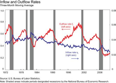
Since 1990, the Bureau of Labor Statistics has estimated labor market flows between employment, unemployment, and “out of the labor force” (nonparticipation). However, because we focus only on the total outflow and inflow rates and want to consider the entire postwar period, we use a method attributed to Shimer (2005) that relies only on characteristics of the level and duration of unemployment. The chart below shows the path of the inflow and outflow rates produced by this method. The inflow rate st (measured on the right axis) spiked up during the recession but has mostly subsided recently. The outflow rate ft (measured on the left axis) reached its lowest level since 1972 during the 2007-09 recession and, despite recent improvements, still stands far below its pre-recession levels.
What Do Flows Tell Us?
An important concept is the flow-consistent unemployment rate (ut*), the level at which the unemployment rate would settle if the inflow and outflow rates stay constant at their current levels. This concept is sometimes called the steady-state unemployment rate, but should not be confused with a natural rate concept. Because flow rates change from month to month, the flow-consistent unemployment rate changes.
The flow-consistent unemployment rate is defined as
 |
The actual and the flow-consistent unemployment rates generally are very close to each other over the postwar period. However, significant deviations have occurred between the two measures during periods of rapid change in labor market conditions. To explain some of the recent large drops in the unemployment rate, we look for periods in which the flow-consistent unemployment rate is far below the actual unemployment rate.
| Historical Unemployment Rate Dynamics | ||||||
| Date | u* | u | u*-u | One-Month Change in u |
Three-Month Change in u |
Twelve-Month Change in u |
| Oct-49 | 5.3 | 7.9 | -2.6 | -1.5 | -0.1 | -2.3 |
| Mar-50 | 5.2 | 6.3 | -1.1 | -0.5 | -0.7 | -2.6 |
| Jul-50 | 4.0 | 5.0 | -1.1 | -0.6 | -0.3 | -1.4 |
| Dec-50 | 3.3 | 4.3 | -0.9 | -0.5 | -0.6 | -0.6 |
| Sep-58 | 6.2 | 7.1 | -0.9 | -0.4 | -0.7 | -1.0 |
| Oct-58 | 5.5 | 6.7 | -1.2 | -0.5 | -0.3 | -0.3 |
| Nov-59 | 4.8 | 5.8 | -1.1 | -0.5 | 0.2 | 1.3 |
| Dec-82 | 9.7 | 10.8 | -1.1 | -0.4 | -0.3 | -2.4 |
| Jun-83 | 8.5 | 10.1 | -1.5 | -0.6 | -0.6 | -1.9 |
| Nov-10 | 8.2 | 9.8 | -1.6 | -0.4 | -0.5 | -0.9 |
| Dec-10 | 8.3 | 9.4 | -1.1 | -0.3 | -0.1 | -0.8 |
| Oct-11 | 7.9 | 8.9 | -1.1 | -0.3 | -0.4 | — |
| Dec-11 | 7.6 | 8.5 | -0.9 | -0.2 | — | — |
The table shows the largest negative deviations between u* and u for the postwar period. When this deviation was at least 0.9 percentage point (the difference in December 2011), the unemployment rate declined 0.5 percentage point on average in the following month. Because our u* calculation uses data from the following month, we expect the deviation would provide such a near-term prediction. But when we look at the change in the unemployment rate over the subsequent three months (fifth column), it declines a further 0.4 percentage point on average. Looking at the subsequent twelve months instead (last column), the unemployment rate declined a further 1.2 percentage points on average. For example, the large June 1983 deviation predicted the subsequent sharp decline in the unemployment rate in early 1984 described in the introductory post to this series.
During the most recent recovery, we have also observed some large deviations between the two measures. The first two were in November and December 2010. As happened previously, these deviations were followed by a substantial decline in the unemployment rate. More recently, in October and December 2011, the flow-consistent unemployment rates were 1.1 and 0.9 percentage points, respectively, below the actual unemployment rate.
A key question is whether this most recent deviation is a clear signal of a further decline in the unemployment rate. The answer depends on whether the behavior of the inflow and outflow rates will be different going forward.
The Importance of the Outflow Rate
While the inflow and outflow rates jointly determine the unemployment rate, historical data show that fluctuations in the outflow rate drive a majority of the fluctuations in the unemployment rate. Economic downturns are typically characterized by short-lived spikes in the inflow rate followed by prolonged weakness in the outflow rate. The inflow rate plays an important role in the rise of the unemployment rate at the onset of recessions, but is typically less important in the decline of the unemployment rate during recoveries (see Elsby, Hobijn, and Şahin [2010]). Historical flow dynamics tell us that unless the economy gets hit with a negative shock that increases job loss, changes in the outflow rate will be the most important determinant of the path of the unemployment rate in the future.
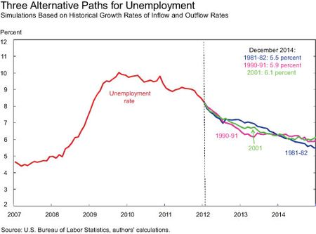
To demonstrate how the improvement in flow rates—especially the outflow rate—can bring down the unemployment rate, we construct a hypothetical unemployment rate path under three scenarios. In these scenarios, we assume the inflow and outflow rates change at the same rate as in the recoveries following the 1981-82, 1990-91, and 2001 recessions. We start the simulations two-and-a-half years from the official NBER trough to ensure that we are comparing similar points of the business cycle. (This simulation is similar to Daly, Hobijn, and Kwok’s simulation computed in 2009 to assess how high the unemployment rate was likely to go.)
In all three scenarios, the unemployment rate declines to around 6 percent by the end of 2014. Indeed if the inflow and outflow rates improve at the same rate as they did in late 1993 and 1994, the unemployment rate will fall to close to 6 percent by early 2013. In contrast, the March 2012 Blue Chip consensus forecast has unemployment remaining above 7.5 percent through 2013.
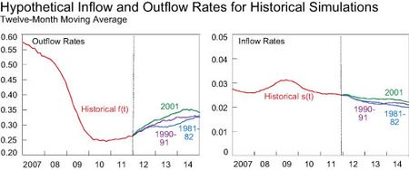
The next chart shows the hypothetical inflow and outflow rates in the three scenarios. Although the decrease in the inflow rate contributes to the decline, the main driver of the decline in the unemployment rate in these scenarios is the improvement in the outflow rate. It is important to note that in all of these scenarios, the increase in the outflow rate is modest: it rises from 25 percent to around 33-34 percent, compared with a peak before the Great Recession of about 60 percent. One concern about these simulations is that with the inflow rate already at very low levels, it may not fall as implied in the simulation. However, even if the inflow rate stays at its current level of 2.3 percent, the outflow rate would only have to rise to 37 percent for the unemployment rate to be at 6 percent by the end of 2014.
What conclusions should we take from this analysis of the bathtub model? First, the future path of the unemployment rate will be determined primarily by movements in the outflow rate. Second, flow dynamics suggest further declines in the unemployment rate. That is because even modest increases in the outflow rate can lead to significant declines in the unemployment rate as long as there is not a big negative shock that triggers a new wave of job
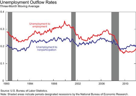
losses. Finally, the unemployment rate can decline regardless of whether workers find jobs or leave the labor force, and thus can fall even in the absence of improved job-finding prospects. In fact, as seen in the last chart, labor market exit has been an important factor in recent movements of the unemployment rate. We will discuss the importance of participation in Friday’s post.
*Christina Patterson is a research associate in the Research and Statistics Group.
Disclaimer
The views expressed in this blog are those of the authors and do not necessarily reflect the position of the Federal Reserve Bank of New York or the Federal Reserve System. Any errors or omissions are the responsibility of the authors.


 RSS Feed
 Follow Liberty Street Economics
That’s a great study. People should really move their feet, and find a job. It’s not easy to live in this world without having resources.
This is exactly the methodology invented at MIT in the late 1950s by Jay W Forrester. He termed it industrial dynamics. It is now termed system dynamics. Please see http://www.systemdynamics.org for more information. This method, sometimes termed ‘bathtub’ dynamics, has been widely used to look at climate change recently and to look at literally hundreds of systems where feedback and time delays are important. John Sterman at MIT has also shown that well educated persons have a difficult time of what is essentially in calculus, integration, when presented with these kinds of problems: rates and accumulation in stocks. Even more so when delay is involved. BTW there are many software packages that implement the system dynamics methodology that would make the mathematics more tractable. In addition they would permit the model to get more complex but perhaps that is the wrong path to take.
Is there a musical chairs going on in the job market. Every month in your bath tub about 5 MM come in and about 5.2 MM go out of the bathtub. Currently there are about 14 MM people in the bath tub, so next month there will be 19 MM however 5.2 will go out leaving behind 13.8 MM. so the number of people in bath tub will depending on how many are coming in and how many are going out. In a year about 60 MM people come in, that is lot of people, about half the working population, that means an employee changes job every 2 years. Well we all know that you and I don’t change job every two years, so some people come many times in the year in this bath tub. This is because? Employers have lot of choice and get rid of people every now and then or there is lot of seasonal jobs or there are lots of jobs in which skill sets can be easily acquired therefore employees can leave or fired and some other person can be hired back again. This to be sounds neither cyclical or structural. However for the people left in the bath tub for more than 1 year, it may be structural and their job skills are no longer required. Don’t know how many people are like that.
Continued…. So probably what is happening is that barring some 1MM (estimate) who really want job and don’t have job, most people who get unemployed are able to find job within one year. Drop in the labor participation is by people, who really don’t need extra money. If job is readily available they will work, if there is hassle to find job, it is not worth looking. These people have sufficient income either from significant other or from their own savings. I am not an economist however if I look all over the world over a period of time, most of the time growth in jobs in the country were not due to monetary policy. Take a look at Germany- their growth is due to increase in export in Emerging market. Brazil- they discovered oil fields in ocean and growth in their commodity business as China grew. Growth in china occurred as they decided to invest in infrastructure and they have cheap labour and multinational companies were able to exploit it, even in US in 1990s it was due to tech investment and increase in productivity, in 2000 it was due to Euphoria created by declining lending standards. In India it happened due to growth in BPO. I have not seen any survey of who these long term unemployed are like their age, gender and skill set. That may help in determining if something can be done to help these people and reduce the unemployment and the mood in the country.
If I take a look at the number of people claiming unemployment claims, it has gone from about 3MM pre recession to 12 MM and now it is about 7 MM. Implying that 5 MM have got job. So these 5MM represents the outflow. Take a look at the unemployment claims for EUC (long term benefits) http://www.oui.doleta.gov/unemploy/euc.asp that number has been declining. Therefore either they have got jobs or have dropped from labor pool. The peak was about 4 MM and now it is 2.8MM Additionally if I look at the distribution of the age group of the people claiming unemployment Majority of them is below the age of 50. If the percentage of people were much higher in the age of 50 or 60 then one of the reasons in the drop in the outflows could have that older people were laid off in higher proportion are not able to find jobs and hence they have dropped out of the labor people. But this does not seem to be the case. Young people college graduates or high school graduates represents the inflow. Even though I hear that they are having difficulty finding jobs, they have student loans and have to repay them. There is a statistic — % of people unemployed for more than 27 weeks and it is at 45% for past few quarters. This number has remained stable, which implies that people unemployed UP to 27 weeks are able to find jobs else they would have graduated to the next category and the ratio would have increased.
It would be helpful to me if you can give me the units for the inflow rate and the outflow rate since the stock is a rate and therefore the inflows and outflows must be a rate over a time period. I assume the unemployment rate is (unemployed people in the Labor force)/Labor force. So is the inflow rate: adds of unemployed/adds to Labor force per time period? Likewise is the outflow rate: loss of unemployed/labor force loss per period? If my thinking is correct, then an increase in the labor force from non-participation if the rate is faster than new employment would result in an increase in the unemployment rate even though the employment picture is getting better. This may be a plausible dynamic if the long term unemployed become encouraged by the prospects of a growing economy.
Wonderful!
In my research I am finding a relationship in the retirement age, or more importantly a change in the retirement age and the unemployment rate. This would relate to your ‘outflow rate’. Later retirement ages seem to hurt the young population the most and I believe that is what we are seeing today.
Thanks guys for fixing the errors. The simple analogy of the bathtub gives me the shivers, honestly.
first, how much of the flows are nonparticipation (6% UE would not been seen as a success with low participation). Second, what variables drive flows (housing will be slower this time, state govts are still contracting unlike previous recessions). predicting the future from the past is tricky business.
So to get back to the connection with Okun’s Law – what is the statistical correlation between the outflow rate and the rate of growth of GDP? Does the bathtub model give us a better estimate of the consequences for unemployment of say 2% growth versus 3% versus 4%?
We also recognized the transcription error in the table and have subsequently revised it so that the correct numbers are now reported.
Some of the numbers in the “Historical Unemployment Rate Dynamics” table seem off (for instance, the third column does not exactly correspond to the difference between the first 2 columns). That could be rounding, but also the sign of the number in the third column seems to be wrong in most instances (it is correct for June 1983).