Creating a History of U.S. Inflation Expectations

Jan J.J. Groen and Menno Middeldorp

Central bankers closely monitor inflation expectations because they’re an important determinant of actual inflation. Treasury inflation-protected securities (TIPS) are commonly used to measure bond market inflation expectations. Unfortunately, they were only introduced in 1997, so historical data are limited. We propose a solution to this problem by using the relationship between TIPS yields and other data with a longer history to construct synthetic TIPS rates going back to 1971.

Using TIPS to Measure Inflation Expectations

The United States, like many other countries, learned the importance of inflation expectations during the 1970s, when employees demanded wage increases to protect themselves against higher inflation, which resulted in businesses passing along increased labor costs in the form of higher prices. Unfortunately, inflation expectations are difficult to measure. One way is to ask people what they expect through surveys. Another is to use inflation-linked bonds.

TIPS are publicly traded government debt securities that compensate investors for the change in consumer prices. So while nominal Treasury holders demand a higher yield to offset expected future inflation, owners of TIPS are willing to accept an initial lower yield. The difference between the nominal yield on ordinary Treasuries and the real yield on TIPS (called the break-even rate) reflects expected inflation. However, nominal bondholders also recognize that actual inflation may deviate from the expected rate and, if they’re risk averse, will also want to be compensated for this uncertainty. In addition, investors care about the liquidity of a security because they don’t like to sell at a discount if they need to unload their holdings. While TIPS offer insurance against inflation, they’re also less liquid than nominal Treasuries; as a result, the break-even rate reflects both inflation risk and liquidity premiums in addition to expected inflation. Nevertheless, the break-even rate is the most commonly used measure of inflation expectations. One reason for this is that bondholders have an incentive to forecast accurately. Another is that break-evens are available in real time. Unfortunately, TIPS aren’t directly useful in helping to understand periods of high inflation, like the 1970s, because they didn’t exist until 1997, and inflation has subsequently been low and relatively stable.

How to Forecast the Past

Fortunately, if we can estimate a relationship between real yields and longer time series and are willing to assume that the relationship is stable over time, then we can use a “backcasting” procedure to construct a TIPS real yields series for earlier time periods. Then we can use historical nominal bond yields to calculate break-even rates. We believe it makes more sense to backcast real yields rather than attempt to estimate historical break-evens directly, because while inflation expectations are unbounded, historical real interest rates are likely closer to levels experienced since 1997.

We select 108 monthly time series dating back to 1971 that are plausibly related to real yields. Nominal yields are at the top of the list because they’re the sum of real yields and inflation expectations. Changes in real yields should thus result in changes in nominal yields. Furthermore, other indicators included in the data set are intended to capture changes in inflation expectations, so together with nominal yields they help identify real yields. The indicators related to inflation expectations are a collection of current price indexes and measures of the output gap. We also include different indicators of economic growth, which should affect real yields. In addition, we include several measures of financial stress, such as credit spreads and realized volatility in financial markets, because in times of financial crisis central banks tend to cut interest rates to cushion the impact on the economy. We include as well a history of private sector expectations from the Philadelphia Fed’s Survey of Professional Forecasters for the GDP deflator (inflation), GDP growth, and the gap between the estimated non-accelerating inflation rate of unemployment (NAIRU) and the actual unemployment rate (a proxy for the output gap).

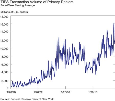
To combine all of those data efficiently in a way that best matches TIPS yields, we use a statistical technique called partial least squares (PLS). The PLS methodology boils the data down into a small number of factors—linear combinations of our variables—that have maximum explanatory power for the TIPS yields. The TIPS yields data since 1997 are then regressed onto the factors to determine coefficients that best combine them into a single estimate. To correct for changes in TIPS market liquidity, which appears to have affected pricing before 2005 and during the financial crisis, we also include the transaction volume of TIPS in the regression (see chart below). We can again use regression analysis since 1997 to obtain loadings—coefficients that relate each individual factor to each of the time series in the data set. The key to our approach is to recognize that we ultimately form a link between the TIPS yields and the data set—the regression coefficients relate the TIPS yields to the factors, while the loadings relate the factors to the data set. Consequently, the product of the loadings and the coefficients allows us to map the data set (either post-1997 or earlier) into historical estimates of TIPS yields.

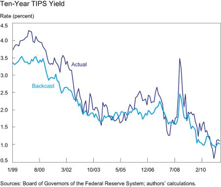
Clearly measuring liquidity in the TIPS market prior to its creation isn’t possible; however, to generate a backcast we need to set a value for TIPS transaction volumes. Simply setting this value to zero would result in a large wedge between the backcasts and the actual TIPS rates in the period immediately after the TIPS bonds started to trade when the market was much less liquid. Instead, we define a level of TIPS transaction volumes that approximates stable market conditions. The aforementioned chart suggests that this was most likely the case between 2005 and mid-2008, as transaction volumes have been substantially more volatile both before and after this period. Therefore, when producing the backcasts we assume that the TIPS transaction volumes are fixed at the average of the period 2005 to mid-2008. This last step completes our backcasting procedure for the ten-year TIPS yield. The next chart presents a comparison between the backcast and actual ten-year TIPS yields. Subtracting the backcast real rates from the historical nominal yields produces break-evens for each of these maturities.

Cross-Checking the Backcast

We can confirm that our synthetic histories are reasonable by comparing them with other available estimates that have long histories.

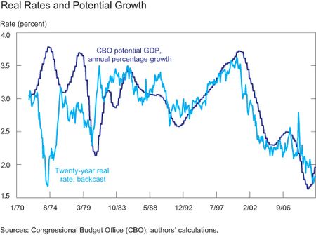
Regarding long-term real rates, theory tells us that these should be related to potential GDP growth. We therefore compare an estimate of potential growth from the Congressional Budget Office with our twenty-year real rate backcast, and find that with the exception of the mid-1970s they track closely (see next chart).

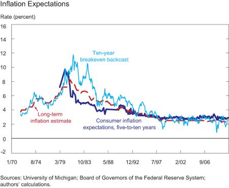
Regarding break-evens, one of these is the University of Michigan’s Survey of Consumer Confidence Sentiment, which has asked for expectations for inflation over five to ten years since 1979. Another is a measure of long-term inflation expectations spliced together from the Survey of Professional Forecasters (from 1990), the Hoey survey of market participants (from 1981 to 1989), and a model of inflation expectations developed by Kozicki and Tinsley (2001) (before 1981). The last chart shows that the ten-year break-even rate tracks these series relatively well, although in the early 1980s the rate appears to be elevated relative to the other measures. This may reflect an elevated inflation risk premium, because there may have been greater uncertainty about the success of the Fed’s inflation-fighting policies.

Overall, the backcast seems to provide a plausible synthetic history of break-evens, allowing for analysis of financial market inflation expectations over a forty-five-year timeframe. Interested readers can download the historical estimates of break-evens here.

Disclaimer
The views expressed in this post are those of the authors and do not necessarily reflect the position of the Federal Reserve Bank of New York or the Federal Reserve System. Any errors or omissions are the responsibility of the authors.

---

Jan J.J. Groen is an officer in the New York Fed’s Research and Statistics Group.

Menno Middeldorp is affiliated with Utrecht University. He was an economist in the New York Fed’s Markets Group when this post was written.