GDP contracted 4 percent from 2008:Q2 to 2009:Q2, and the unemployment rate peaked at 10 percent in October 2010. Traditional backward-looking Phillips curve models of inflation, which relate inflation to measures of “slack” in activity and past measures of inflation, would have predicted a substantial drop in inflation. However, core inflation declined by only one percentage point, from 2.2 percent in 2007 to 1.2 percent in 2009, giving rise to the “missing deflation” puzzle. Based on this evidence, some authors have argued that slack must have been smaller than suggested by indicators such as the unemployment rate or deviations of GDP from its long-run trend. On the contrary, in Monday’s post, we showed that a New Keynesian DSGE model can explain the behavior of inflation in the aftermath of the Great Recession, despite large and persistent output gaps. An implication of this model is that information about the future stance of monetary policy is very important in determining current inflation, in contrast to backward-looking Phillips curve models where all that matters is the current and past stance of policy.
In the New Keynesian DSGE model, inflation depends on a measure of slack and on expected inflation. In turn, expected inflation is determined by expected future marginal costs. Putting the two things together, today’s inflation depends on current and expected future marginal costs. According to the model, inflation did not fall much during the recession because expectations of future marginal costs, and therefore inflation expectations, remained anchored. In other words, marginal costs were expected to revert back to their normal level even though current marginal costs were low.
This raises the question of what determines the expected reversion of marginal costs. In our paper “Inflation in the Great Recession and New Keynesian Models,” we show that if the prices of individual goods are sufficiently sticky, then monetary policy can have substantial effects on future marginal costs and therefore on inflation. Specifically, if the central bank is committed to stabilize inflation around its target, then it will lower its policy rate and indicate that it will maintain it at a low level for an extended period of time when output is below potential. This announcement tends to lower longer-term rates, which stimulates consumption and investment demand, and in turn raises expectations of future marginal costs.
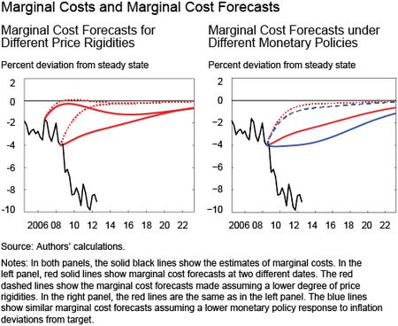
To see why the degree of price stickiness matters, the left panel of the chart below shows the actual path of marginal costs that are not directly observed but are inferred by the model, along with the forecasts by the agents in the model at two different points in time. The solid red lines are forecasts using our estimated value of the degree of price stickiness, and the dashed lines are forecasts using a lower estimate of price stickiness from the well-known paper by Smets and Wouters. The chart shows that if prices are relatively flexible, marginal costs revert quickly to their steady state. In contrast, marginal costs revert slowly to their steady state when prices are sticky. Since in New Keynesian models inflation is determined by the present value of future marginal costs, this finding implies that with flexible prices, current marginal costs largely drive inflation (the intuition being that firms quickly lower prices in line with current marginal costs). Conversely, with sticky prices, the entire future path of marginal costs becomes relevant for inflation determination as firms take into account future marginal costs when setting current prices.
If prices are sufficiently sticky, monetary policy has a considerable impact on the dynamics of marginal costs. To substantiate this claim, the right panel of the above chart shows marginal cost forecasts under two different assumptions about the policy response to deviations of inflation from its target. The red lines show the marginal cost forecasts under the baseline behavior of policy. The blue dash-and-dotted lines instead assume that the central bank responds less to inflation deviations from target. This weaker policy response to inflation makes little difference to the expected path of marginal costs with flexible prices since marginal costs revert back to their steady state regardless of the conduct of monetary policy. However, with price stickiness, the marginal cost forecasts become very sensitive to the central bank’s reaction to inflation movements. Thus, if prices are sticky, the path of expected future marginal costs can be more effectively controlled by a monetary policy that reacts strongly to inflation. As a result, monetary policy is still able to anchor inflation expectations and therefore current inflation.
It has been argued that it is harder for central banks to affect inflation when inflation is unresponsive to current slack, that is, when the Phillips curve is flat. For instance the 2013 IMF World Economic Outlook asks, “Does Inflation Targeting Still Make Sense with a Flatter Phillips Curve?” Seen from the perspective of our model, a flatter Phillips curve does not imply that monetary policy control is diminished. On the contrary, by affecting future marginal costs, monetary policy can effectively anchor inflation expectations, which is why, in our story, inflation did not fall in the Great Recession.
Disclaimer
The views expressed in this post are those of the authors and do not necessarily reflect the position of the Federal Reserve Bank of New York or the Federal Reserve System. Any errors or omissions are the responsibility of the authors.
Marco Del Negro is an assistant vice president in the Federal Reserve Bank of New York’s Research and Statistics Group.
Marc Giannoni is an assistant vice president in the Research and Statistics Group.
At the time this post was written, Raiden B. Hasegawa was a senior research analyst in the Research and Statistics Group.
Frank Schorfheide is a professor of economics at University of Pennsylvania.


 RSS Feed
 Follow Liberty Street Economics
The point of these two posts is to test a theory of aggregate inflation determination and to show that this theory performs reasonably well. We are well aware of the large literature on the determination of individual prices, both at the firm level and item level. The challenge has been to relate individual price adjustments to the evolution of aggregate prices: knowing a lot about how widget prices are set is unfortunately not always informative for aggregate inflation, which is what we care about in these posts. Our two posts perform a very concrete exercise: they document the outcome of a forecasting exercise for inflation and output growth. We show that as of 2008, the model did predict fairly accurately the subsequent behavior of these variables. This suggests that the model provides some value to understanding what is happening in this important area.
It’s important to point out, in response to Tim Young’s post, that the Fed is not funded by taxpayers. In fact, the Fed earns money, which it then gives to the US Treasury.
I followed the link across from FT Alphaville to what seemed like a promising article and was disappointed. To cut through the academic gobbledegook, all you seem to be saying is that, you have demonstrated, via a mathematical model, that if prices are difficult to move, and if the central bank is expected to be ensure that prices will be rising at its inflation target in the not-too-distant future, it is not worth going to the trouble of cutting prices now. I am sorry to be rude, but without some fieldwork gathering some evidence that this is actually how business reached its price-setting decisions, this seems to me like mere internal hypothesising, which with all due respect to the authors, is probably little informed by practical experience of how business works. I can see why the key involvement of public faith in the Fed’s ability to meet its inflation objective in this thinking goes down well at the Fed though. If I were a US taxpayer, I would wonder why I am paying for such detached theorising to be done in what must be some of the most expensive real estate in the US.
right, by the other side of the coin is that in your model agents must have been expecting output gaps to close quickly! ah!