Household Consumption Mobility over the Life‑Cycle

Giacomo De Giorgi and Nicole Dussault

Editors’ note: The y-axis labels on the charts in this post have been corrected to read “Share,” rather than “Percent.”

Commonly used metrics of inequality and mobility attempt to capture how household (or individual) income compares to the rest of the population and how persistent that income is over the life cycle. It can be helpful to think of the income distribution as a ladder—each household is a rung, ranked by its level of income. If household income rankings remain constant over time, this could indicate a low level of mobility in a society. However, income only constitutes one aspect of overall well-being. Another crucial, and potentially more appropriate, dimension is consumption expenditures—how much do people spend on goods and services? In many ways, consumption can be thought of as a proxy for quality of life, since what a household buys says a lot about its access to the necessities of life. Therefore, the analysis of consumption expenditures mobility constitutes a crucial dimension of mobility.

So if we rank households in a ladder based on their consumption levels, how persistent are these rankings over the life-cycle? Is persistence different across high and low levels of consumption? Further, does consumption mobility vary between different demographic groups? These are the questions we address in this post as well as in a broader research agenda. We investigate how likely households are to remain at the top or the bottom of the consumption spending distribution. We look at overall mobility and, as an example of differences across demographic groups, mobility broken down by race.

The PSID

For our analysis, we use the Panel Study of Income Dynamics (PSID) to construct three decades of household level life-cycle consumption profiles, beginning in 1981. While we pick 1981 as our base year for convenience in terms of sample size, our findings are robust to the choice of the base year.

The PSID is a longitudinal survey conducted by the University of Michigan, which has continuously surveyed households since 1968. Members of households from the 1968 survey became PSID “sample members” and were surveyed annually until 1997, after which they were surveyed biannually. Furthermore all lineal descendants of original sample members became sample members themselves and were independently followed and surveyed once they started their own households.

While most information in the PSID is gathered at the household level, some data is available at the individual level. In our analysis we only include heads of households, since they have the most consistent information over the entire survey, while taking into account the household structure—the number and characteristics of dependents. Since the PSID assigns one head per household, our analysis is therefore effectively at the household level.

Historically the PSID asked respondents to report the monetary value of their household’s consumption of food at home, food away from home, and food stamps—with the exceptions of 1973, 1988 and 1989. Then beginning in 1999, households have been asked to detail their spending on a wide array of goods and services, such as utilities, transportation costs, and healthcare. Unfortunately, spending on clothing, vacations, entertainment, and other similar discretionary spending only became available in 2005.

Measuring Household Consumption Expenditures

Only a limited amount of consumption spending information is available prior to 1999, so we use a consumption imputation method developed by Blundell, Pistaferri, and Preston. This enables us to predict a household’s consumption in each sample year, based off a series of covariates that are available in every year of the survey. Specifically, the method uses spending on food, socio-demographic information (state, age, number of children, highest level of education, marital status, disability, etc.), and price controls to predict nonfood consumption. Our final measure of consumption expenditures includes food, rent equivalents, home insurance, electricity, heat, water/sewage, miscellaneous utilities, car insurance, gas, parking, bus/train, cabs, other transport, school fees, other school costs, childcare, health insurance, hospital care, doctors, and drugs. We then adjust the predicted household consumption each year by the Consumer Price Index and the OECD equivalence scale to arrive at annual measures of real consumption that take into account both the number and ages of all household members.

Consumption Mobility

For each survey year, we order all households by consumption levels and divide them into quintiles—brackets each containing 20 percent of the households, based on their ranking in the consumption ladder. Our analysis then mimics the method of transition matrices, in a standard regression framework, to assess life-cycle consumption mobility. In this analysis we focus on two initial quintiles—the bottom and the top. In other words, we will describe the probability that a household first observed in the bottom quintile stays in the bottom quintile, and the probability that a household that begins at the top, stays at the top. Although the analysis of average mobility—the persistence in any given quintile—is interesting as well, it could mask important heterogeneity for the two natural focal quintiles: bottom and top.

We set 1981 as a base year, using households present in the PSID at that time whose heads identify as black or white as our fixed sample. We then analyze the transition probabilities for each household for every survey year up to 2011. Therefore, we are able to capture a substantial part of the life-cycle, as our typical head of household is 40 years old in 1981.

The Aggregate Picture

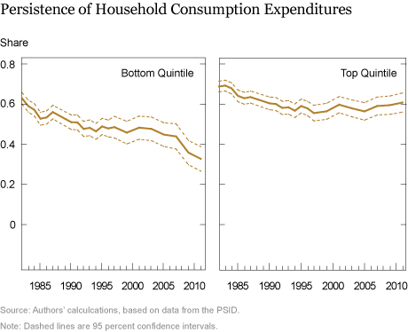
In the chart below, we draw the probability of a household remaining in the bottom or top quintile (left and right panel respectively), of the national consumption distribution for each year, given that a household is observed in that particular quintile in 1981.

Persistence in the Bottom Quintile

The probability of the average PSID household being observed in the bottom quintile, after having been observed there in 1981, drops continuously over the life-cycle. While there is an initial drop to about 63 percent between 1981 and 1982, that probability declines steadily to about 33 percent by 2011. This tells us that of the surviving households observed for thirty years, slightly more than a third of those originally observed in the bottom quintile in 1981 remain in that quintile in 2011. On the other hand, this also suggests quite a bit of upward mobility. The other two-thirds of the 1981 bottom quintile move up in the national ranking by 2011 (with about 27 percent, 16 percent, 15 percent, and 9 percent in the second, third, fourth, and fifth 2011 quintiles, respectively).

Persistence in the Top Quintile

The right panel of the chart above draws the time series of the probability of a household remaining in the top quintile if observed there in the base year. The chart tells us that after an immediate exit from the top quintile (about 30 percent of households drop out of the top quintile just one year after the initial observation), the probability of remaining in the top quintile stays rather constant over the course of three decades and tapers off to about 60 percent. This suggests a higher life-cycle persistence in the top end of the distribution.

Black and White Mobility

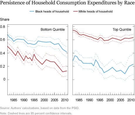
Our next step is to perform the same analysis separately for households with a head of household who identifies as black or white, while preserving their consumption ranking relative to the pooled ranking. This way, we can see how the probability of staying in the bottom or top quintile varies for different racial groups. Again, since we only use data on heads of households and consumption is reported for family units, our analysis is effectively at the household level. We denote the estimates with a blue and red solid line for black heads of household and white heads of household respectively. The dashed lines represent 95 percent confidence intervals around the estimated parameters.

The above chart shows a marked difference in the transition probabilities for households in the bottom quintile (left panel). Black heads of households (blue line) tend to remain in the bottom quintile with a significantly higher probability than white heads of households (red line). However the pattern is reversed for top-quintile persistence (right panel): White heads of households are much more likely to remain at the top of the distribution. What is striking is the magnitude of the differences between these two groups, particularly for the top end of the distribution: White heads of households are about twice as likely to remain at the top over their life-cycle.

Accounting for Observables

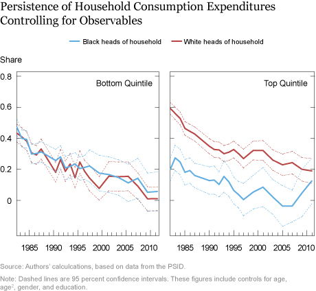
The analysis so far, however, doesn’t account for differences in observable characteristics between black and white heads of households. This is exactly the analysis we present in the chart below. We again estimate the transition probabilities, this time adding controls for age, age squared, gender, and the highest level of education of the head of household, fully interacted with race. We note that given the conditional analysis here, the probability levels drawn are not expected to match the levels of the unconditional profiles in the previous charts.

Persistence in the Bottom Quintile Controlling for Observables

The differential probabilities of a household remaining in the bottom quintile appear to be fully eliminated by our sets of controls. In particular, we note that black households at the bottom of the consumption distribution in our sample are larger in size, more likely to be headed by a single female head of household, and have lower levels of education.

Persistence in the Top Quintile Controlling for Observables

While we have shown that the probabilities of remaining in the bottom quintile are essentially the same for black and white heads of households, once basic socio-demographic characteristics are accounted for, the same is not true for the top quintile. In fact, as we can clearly see from the right panel of the above chart, those differentials are still present, albeit diminished, when we control for observable characteristics. Although the differential in probabilities tends to fade out over the life-cycle they are quite large for the first two decades, with white households almost twice as likely to remain in the top quintile. This suggests that whites’ persistence in the top consumption quintile is much higher than blacks’ persistence, even when comparing observationally equivalent households in terms of the age, education, and gender of the head of household. It is important to note that there could be a number of other characteristics that differ between the two groups. In particular, we observe that black heads of household at the top end of the consumption distribution appear to have lower, and importantly more volatile (over the life-cycle), incomes than white heads of household.

Summary

We conclude that black and white PSID heads of household appear to have different life-cycle consumption mobility profiles on average, with black households generally having a higher persistence at the bottom of the distribution and a lower persistence at the top. The immobility at the bottom seems to be fully explained by a small set of important characteristics. At the same time, those characteristics fail to account for the larger downfall risk experienced by black heads of household at the top end of the distribution.

Upon further investigation, we note that black heads of household in the PSID are clustered in lower paying occupations, even within an industry. Importantly, black heads of household are substantially more likely to appear in occupations that feature high wage dispersion, which could indicate a higher volatility in income and therefore higher risk of downfall. It is also possible that the permanent and transitory component of the shocks to earnings could be rather different between black and white households, with blacks having a much less permanent income profile at the top of the distribution. These latter facts call for further research and certainly a deeper investigation of the income generating process.

Disclaimer

The views expressed in this post are those of the authors and do not necessarily reflect the position of the Federal Reserve Bank of New York or the Federal Reserve System. Any errors or omissions are the responsibility of the authors.

---

Giacomo De Giorgi is a senior economist in the Federal Reserve Bank of New York’s Research and Statistics Group.

Nicole Dussault is a senior research analyst in the Bank’s Research and Statistics Group.

How to cite this blog post:

Giacomo De Giorgi and Nicole Dussault, “Household Consumption Mobility over the Life-Cycle,”
Federal Reserve Bank of New York Liberty Street Economics (blog), May 11, 2016,
http://libertystreeteconomics.newyorkfed.org/2016/05/household-consumption-mobility-over-the-life-cycle.html.