The years following the Great Recession were challenging for forecasters for a variety of reasons, including an unprecedented policy environment. This post, based on our recently released working paper, documents the real-time forecasting performance of the New York Fed dynamic stochastic general equilibrium (DSGE) model in the wake of the Great Recession. We show that the model’s predictive accuracy was on par with that of private forecasters and proved to be quite a bit better, at least in terms of GDP growth, than that of the median forecasts from the Federal Open Market Committee’s (FOMC) Summary of Economic Projections (SEP).
Comparing Forecast Accuracy
Unlike some other deep downturns, the Great Recession was not followed by a swift recovery, but instead generated a sizable and persistent output gap. This output gap, however, was not accompanied by deflation, as a traditional Phillips curve would have predicted. Additionally, the policy environment was unprecedented, with the nominal federal funds rate pinned to the zero lower bound for years and the Federal Reserve relying extensively on unconventional monetary policy and forward guidance.
The unusual conditions in the aftermath of the recession presented a challenging environment for any econometric model to process. DSGE models, often criticized for their unrealistic assumptions (and often rightly so), must surely have been at a disadvantage. So how did ours fare?
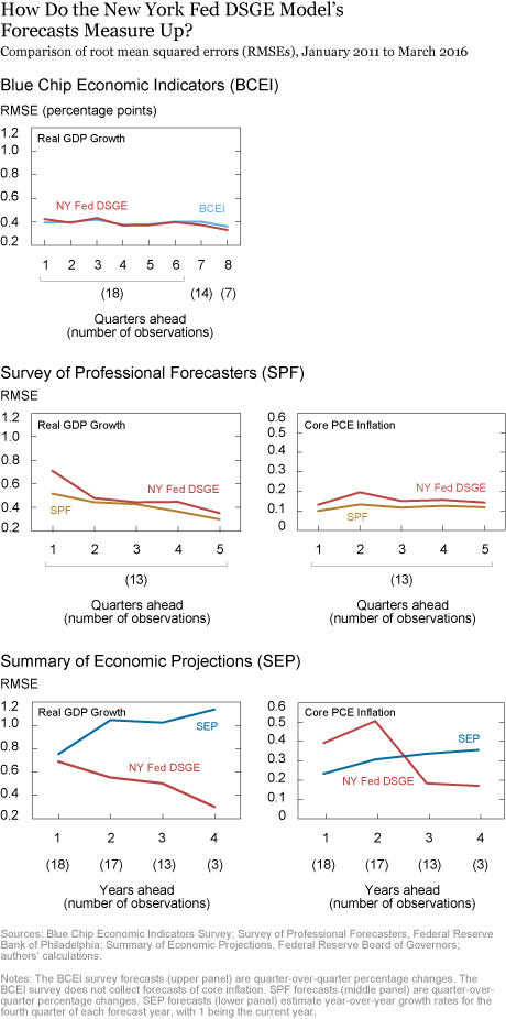
The chart below compares the root mean squared errors (RMSEs), a standard measure of forecast accuracy, of the New York Fed DSGE model’s output growth and core PCE inflation forecasts against those of the Blue Chip Survey of Economic Indicators (BCEI), the Survey of Professional Forecasters (SPF), and the SEP. We examine RMSEs from 2011, when we started forecasting, through early 2016, giving us enough data to compare the forecasts against actual outcomes. Each panel has the forecast horizon on the x-axis and the corresponding RMSE on the y-axis. So, for instance, the blue line in the upper left panel shows the RMSE of BCEI GDP growth forecasts at each horizon, from one quarter ahead to eight quarters ahead.
Before describing the results, we should stress a couple of things. First, this is not some sort of ex post exercise like the one done, for example, in this paper. These forecasts were actually produced and published at the time—originally in internal documents, then, since mid-2014, on the Liberty Street Economics blog (here is our latest forecast). Second, for this comparison we always picked the New York Fed DSGE forecast preceding a given private sector forecast (and contemporaneous with the SEP forecast), so that the DSGE model was, if anything, at an informational disadvantage.

In the chart above, the upper panel shows that the DSGE’s forecast errors for output growth pretty much match the consensus BCEI’s over an eight-quarter horizon, indicating that the DSGE’s forecast accuracy is comparable to that of the consensus Blue Chip. (The BCEI does not include forecasts of core inflation.) In the middle panel, the DSGE’s RMSEs are a little larger than the SPF’s for both output and inflation, but the differences are small. (We should stress that the SPF often has a substantial informational advantage, as its forecasts are made right after the first GDP release, while the DSGE forecasts are, in many cases, made right before it.)
The most striking comparison, shown in the lower panel, is the one with the median SEP forecast. Note that in the case of the SEP the horizontal axis measures years, as opposed to quarters (year 1 being the current year). It is clear that the New York Fed DSGE model forecasted output growth much more accurately than the median SEP, especially at longer horizons. The DSGE performed worse at forecasting inflation than the median SEP up to a two‑year horizon, but outperformed the SEP at a three‑year horizon.
Financial Shocks and the Great Recession
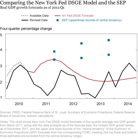
What explains the DSGE model’s greater forecast accuracy for output growth versus the SEP? The chart below shows the New York Fed DSGE forecast of four-quarter GDP growth from early 2011 (red line), together with the data available at the time (dotted black line). For comparison, we also include the contemporaneous 2011 SEP projection (blue markers; we show the upper and lower bounds of the SEP’s “central tendency,” which includes all SEP participants’ projections except the top and bottom three), and the actual data as of November 2017 (solid black line). We see that the SEP projected a relatively quick recovery from the Great Recession, with growth rates above four percent. The U.S. economy had rebounded quickly from previous deep recessions, and so a widely shared view held that it would rebound from the Great Recession as well. The New York Fed DSGE model instead projected a very slow recovery from the financial crisis, which we now know was much closer to the realized growth trajectory.
What was the basis for this sluggish-growth prediction? Our DSGE model features financial frictions and, as we have shown elsewhere, it attributes the Great Recession to financial shocks. According to the model, these shocks have a very persistent effect on the economy. Put the two together and you obtain a forecast for a slow recovery from the financial crisis, a finding that echoes the results of Reinhart and Rogoff, although it was obtained in a completely different setting. (By the way, this was also our rationalization for the New York Fed DSGE forecast included in a June 2011 FOMC memo that was recently made public. As we wrote then: “Forecasts in the FRBNY model are mainly driven by the negative headwinds from the financial crisis.”)

The fact that New York Fed DSGE forecasts were more accurate than those of the SEP, at least for output growth, during the recovery is interesting in light of the pushback that DSGE models suffered after the Great Recession. DSGE models were criticized for their inadequacy during the financial crisis (there was even a congressional hearing about it!). While that criticism was in many ways warranted in that most (if not all) DSGEs developed before the crisis were useless in terms of understanding many aspects of the crisis, this exercise shows that some later models, including the New York Fed DSGE model, got one thing right: the transmission of the financial shock to the macroeconomy.
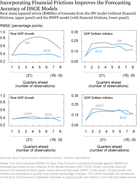
How can we be sure that financial frictions are the main reason for our DSGE model’s forecasting accuracy? To address this question, we compare the forecasts generated by the canonical Smets-Wouters DSGE model (the SW model) to those generated by the same model augmented with financial frictions (the SWFF model). This comparison gets to the heart of why our DSGE model, a more complex version of the SWFF model, performed well in the post-crisis period. The figure below shows that the RMSEs obtained from the SWFF model (lower panel) are close to those of the Consensus Blue Chip for both GDP growth and GDP deflator inflation. Most importantly, it shows that removing financial frictions (SW, upper panel) dramatically worsens the forecasting performance, especially for GDP growth.

Why does forecasting performance decline when financial frictions are not factored in? Because the SW model attributes the Great Recession to transitory disturbances, it expects the economy to make a faster return to normal conditions—that is, for the output gap to close quickly. And when it turns out that the gap does not close, the SW model attributes this forecast error to additional temporary negative shocks, with the consequence that it continually predicts overly optimistic growth, leading to a poor overall forecasting performance.
In conclusion, we have documented the accuracy of the projections of the New York Fed DSGE model during the recovery from the financial crisis. We find that in the short and medium run—one to eight quarters ahead—our DSGE model’s RMSEs are comparable to those obtained from the mean and median forecasts of the Blue Chip and SPF surveys, respectively. However, relative to the median of the FOMC’s Summary of Economic Projections, the New York Fed DSGE model produced much more accurate output growth forecasts, especially at longer horizons. On inflation, the New York Fed DSGE model performed worse than the median SEP up to a two-year horizon, but performed better than the SEP at a three-year horizon. We find that financial frictions play a major role in explaining these results, especially in terms of the projections for economic activity, since they imply a slow recovery from financial crises.
Disclaimer
The views expressed in this post are those of the authors and do not necessarily reflect the position of the Federal Reserve Bank of New York or the Federal Reserve System. Any errors or omissions are the responsibility of the authors.
 Michael Cai is a senior research analyst in the Federal Reserve Bank of New York’s Research and Statistics Group.
 Marco Del Negro is a vice president in the Bank’s Research and Statistics Group.
 Marc Giannoni is director of research at the Federal Reserve Bank of Dallas.
 Abhi Gupta is a senior research analyst in the Federal Reserve Bank of New York’s Research and Statistics Group.
 Pearl Li is a senior research analyst in the Bank’s Research and Statistics Group.
How to cite this blog post:
Michael Cai, Marco Del Negro, Marc Giannoni, Abhi Gupta, and Pearl Li, “Forecasts of the Lost Recovery,” Federal Reserve Bank of New York Liberty Street Economics (blog), May 9, 2018, http://libertystreeteconomics.newyorkfed.org/2018/05/forecasts-of-the-lost-recovery.html.


 RSS Feed
 Follow Liberty Street Economics