Assessing Contagion Risk in a Financial Network

Fernando M. Duarte, Collin Jones, and Francisco Ruela

In compiling a list of key takeaways of the 2008 financial crisis, surely the dangers of counterparty risk would be near the top. During the crisis, speculation on which financial institution would be next to default on its obligations to creditors, and which one would come after that, dominated news cycles. Since then, there has been an explosion in research trying to understand and quantify the default spillovers that can arise through counterparty risk. This is the first of two posts delving into the analysis of financial network contagion through this spillover channel. Here we introduce a framework that is useful for thinking about default cascades, originally developed by Eisenberg and Noe.

A Financial Network with Contagion

We start by envisioning financial firms as nodes in a network. The connections between nodes represent firms’ net borrowing (that is, borrowing minus lending) from one another. There is a connection from node A to node B if A is a net lender to B. In addition, nodes can borrow from and lend to the broader economy, which we call the outside sector.
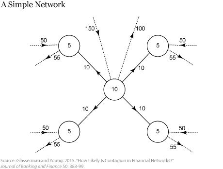
The illustration below, taken from Glasserman and Young (ungated version here), shows an example of a simple network. The four arrows originating in the central node and pointing into the four peripheral nodes show that the central node owes 10 to each of the peripheral nodes. In other words, the central node is a net borrower from each of the other nodes. The peripheral nodes have no net borrowing or lending among themselves. For this network, we then say that the central node has inside liabilities of 40, while each peripheral node has inside assets of 10.

In addition to its claims inside the network, the central node has borrowed 100 from, and has lent 150 to, the outside sector, depicted by the dashed lines with arrows going out of and into the central node. The central node therefore has 100 in outside liabilities and 150 in outside assets.
The difference between all assets and all liabilities gives each node’s net worth. The central node has a net worth of 10, shown inside the circle that represents the node.
Each peripheral node has outside assets of 50, outside liabilities of 55, and inside assets of 10 with respect to the central node, for a net worth of 5.

Initial Losses and Propagation

The action starts when some losses occur. We assume that initial losses occur in the outside sector. One example of such a loss is an increase in defaults on residential mortgages held by banks.

For sufficiently high initial losses, some nodes in the network will be unable to pay their creditors—the other nodes and the outside sector—in full. The first dominoes have fallen. All debts for the defaulting nodes, including those outside the network, are written down pro rata (proportionally) and creditors receive only a fraction of their promised payments. Note that under a pro rata allocation, nodes default on either all of their creditors or none of them. When creditors for some node are not paid in full, they may themselves be unable to pay their own creditors. The losses stemming from a defaulting counterparty can in turn trigger further defaults at other institutions, giving rise to a default cascade. Initial losses thus get propagated and amplified inside the network.

To understand how this works, let’s see what happens when the outside assets of the central node in our first illustration have losses of size 94. Outside assets for this central node decrease from 150 to 56. Total liabilities are initially 140. After the initial losses, under a pro rata allocation, each liability is cut to 40 percent as the central node only has 56 remaining in assets. Each peripheral node is left with 54 assets and 55 liabilities, enough to pay most of their liabilities, but not enough to avoid default on some obligations.

We follow the definition of systemic loss put forth by Glasserman and Young as “the total loss in asset values summed over all entities in the system.” In this calculation, the total losses would be 182 (94 + 84 + 1 * 4). Note that any shock larger than 80 would have caused a default cascade, but any shock larger than 10 would have led to amplified loss.

Connections and Amplification

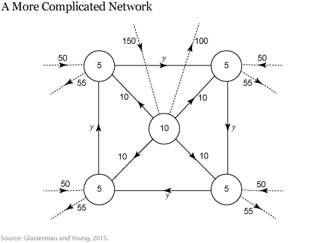
The next illustration shows a more complicated network, depicting the same network as before except that now there is a cycle of obligations of size y connecting the peripheral nodes. Now, if the central node loses more than 80 in its outside assets after some shock, there is a more severe default cascade. Each peripheral node defaults not only on its creditors outside the network, but also on one of its peripheral neighbors. If we assume the initial shock to the central node is 94 and y is equal to 10, we can compute the final value of the inside liabilities of the peripheral nodes after the shock has fully spread through the network. All peripheral nodes default and the total losses to the system equal 182.73, which is again greater than the value of the initial shock. (We leave the details of the calculation to the reader!)

Several other factors can exacerbate the economic losses of default cascades beyond the simple domino default spillovers, including delay of payments, inefficient liquidations, penalties, legal fees, and, more generally, disruptions to the provision of financial intermediation services to the real economy.

The Disconnected Network

To quantify the losses stemming from the network structure, as opposed to the initial losses, we compare losses for the system (the network plus the outside sector) to the losses in a hypothetical system in which all connections inside the network have been severed. This hypothetical disconnected system has all connections between nodes inside the original network removed, but the links with the outside sector intact. We also assume that the net worth at each node remains unchanged by creating, for each node, a fictitious claim to the outside sector equal in value to the net value of all the connections that were removed. Depending on the sign of the net value of removed connections, the new fictitious claim can be an asset or a liability. If it is an asset, we assume it is not subject to the initial shock that affected the outside assets to keep the initial losses identical to that of the original network. If the new fictitious claim is a liability, we assume it has the same priority as all other liabilities. In case of default, the new fictitious liability gets haircut pro rata like all other non-fictitious liabilities.

Given the same initial shock of 94, only the central node would default in a disconnected network—meaning the losses to the system would be equal to the value of the initial shock (94) plus the shock minus the original wealth of the defaulting node (94 − 10), for a total of 178 (94 + 84). The ratio of losses under the connected system to losses under the disconnected system provides a natural answer to the question “how important is the network?” We can see that this ratio equals 2.3 percent ((182 − 178)/178) in our first example and 2.66 percent ((182.73 − 178)/178) in the second example. The higher loss ratio in the second case reflects the fact that it involves a more connected network.

Hypothetical Scenarios

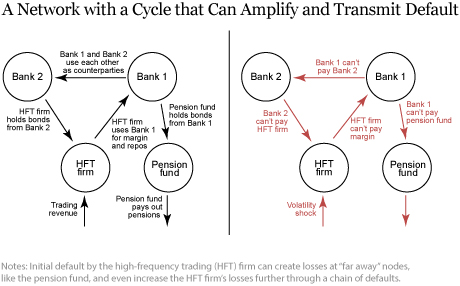
We can also use the framework to think about future hypothetical scenarios. The next illustration shows a scenario featuring bank, high-frequency trading (HFT) firm, and pension fund counterparties as one example of a potential trading network. We pick this example to highlight that very disparate parts of the financial system that are not directly connected and seemingly unrelated—such as arcane HFT firms and pension funds used by millions—can impose spillovers on each other even over two or more degrees of separation. Suppose that we observe an unexpected decline in the price of stocks that causes large initial losses for the HFT firm but no losses at the other nodes of the network. If the losses are large enough, the HFT firm is forced to default on its obligations to Bank 1. If the default on Bank 1 is substantial enough, Bank 1 must default as well, imposing losses on Bank 2 and the pension fund. Losses at Bank 2 can, in turn, create further losses for the HFT firm, triggering a new round of defaults. This also means that the losses to the pension fund continue to be amplified due to the network’s structure.

One can see how financial stress can easily propagate through the system and affect firms that are “far away” from the original shock. But how bad might these default cascades be in practice? Find out in our next post, which features an empirical analysis tracing the bounds of default spillovers for the U.S. financial system.

Fernando M. Duarte is an economist in the Federal Reserve Bank of New York’s Research and Statistics Group.

Collin Jones is a former senior research analyst in the Bank’s Research and Statistics Group and a Ph.D. student in economics at University of California, Berkeley.

Francisco Ruela is a senior research analyst in the Bank’s Research and Statistics Group.

How to cite this post:

Fernando M. Duarte, Collin Jones, and Francisco Ruela, “Assessing Contagion Risk in a Financial Network,” Federal Reserve Bank of New York Liberty Street Economics, June 24, 2019, https://libertystreeteconomics.newyorkfed.org/2019/06/assessing-contagion-risk-in-a-financial-network.html.

---

Disclaimer

The views expressed in this post are those of the authors and do not necessarily reflect the position of the Federal Reserve Bank of New York or the Federal Reserve System. Any errors or omissions are the responsibility of the authors.