The availability of large data sets, combined with advances in the fields of statistics, machine learning, and econometrics, have generated interest in forecasting models that include many possible predictive variables. Are economic data sufficiently informative to warrant selecting a handful of the most useful predictors from this larger pool of variables? This post documents that they usually are not, based on applications in macroeconomics, microeconomics, and finance.
Nowadays, a researcher can forecast key economic variables, such as GDP growth, using hundreds of potentially useful predictors. In this type of “big data” situation, standard estimation techniques—such as ordinary least squares (OLS) or maximum likelihood—perform poorly. To understand why, consider the extreme case of an OLS regression with as many regressors as observations. The in-sample fit of this model will be perfect, but its out-of-sample performance will be embarrassingly bad. More formally, the proliferation of regressors magnifies estimation uncertainty, producing inaccurate out-of-sample predictions. As a consequence, inference methods aimed at dealing with this curse of dimensionality have become increasingly popular.
These methodologies can generally be divided into two broad classes. Sparse modeling techniques focus on selecting a small set of explanatory variables with the highest predictive power, out of a much larger pool of possible regressors. At the opposite end of the spectrum, dense modeling techniques recognize that all possible explanatory variables might be important for prediction, although the impact of some of them will likely be small. This insight justifies the use of shrinkage or regularization techniques, which prevent overfitting by essentially forcing parameter estimates to be small when sample information is weak.
While similar in spirit, these two classes of approach might differ in their predictive accuracy. In addition, a fundamental distinction exists between a dense model with shrinkage—which pushes some coefficients to be small—and a sparse model with variable selection—which sets some coefficients to zero. Sparse models are attractive because they may appear to be easier to interpret economically, and researchers are thus more tempted to do so. But before even starting to discuss whether these structural interpretations are warranted—in most cases they are not, given the predictive nature of the models—it is important to address whether the data are informative enough to clearly favor sparse models and rule out dense ones.
Sparse or Dense Modeling?
In a recent paper, we propose to shed light on these issues by estimating a model that encompasses both sparse and dense approaches. Our main result is that sparse models are rarely preferred by the data.
The model we develop is a variant of the so-called “spike-and-slab” model. The objective of the analysis is forecasting a variable—say, GDP growth—using many predictors. The model postulates that only a fraction of these predictors are relevant. This fraction—which is unknown and is denoted by q—is a key object of interest since it represents model size. Notice, however, that if we tried to conduct inference on model size in this simple framework, we would never estimate it to be very large. This is because of the problem of having too many variables relative to the number of observations, as discussed above. Therefore, to make the sparse-dense horse race fairer, it is essential to also allow for shrinkage: whenever a predictor is deemed relevant, its impact on the response variable is prevented from being too large, to avoid overfitting. We then conduct Bayesian inference on these two crucial parameters—model size and the degree of shrinkage.
Applications in Macro, Finance, and Micro
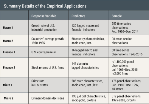
We estimate our model on six popular “big” data sets that have been used for predictive analyses in the fields of macroeconomics, finance, and microeconomics (see Section 3 of the paper linked above for more information about these data sets). In our macroeconomic applications, we investigate the predictability of U.S. industrial production and the determinants of economic growth in a cross section of countries. In finance, we study the predictability of the U.S. equity premium and the cross-sectional variation of U.S. stock returns. Finally, in our microeconomic analyses, we investigate the decline in the crime rate in a cross section of U.S. states and eminent domain decisions. The table below reports some details of our six applications, which cover a broad range of configurations, in terms of types of data—time series, cross section, and panel data—and sample sizes relative to the number of predictors.

Result #1: No Clear Pattern of Sparsity
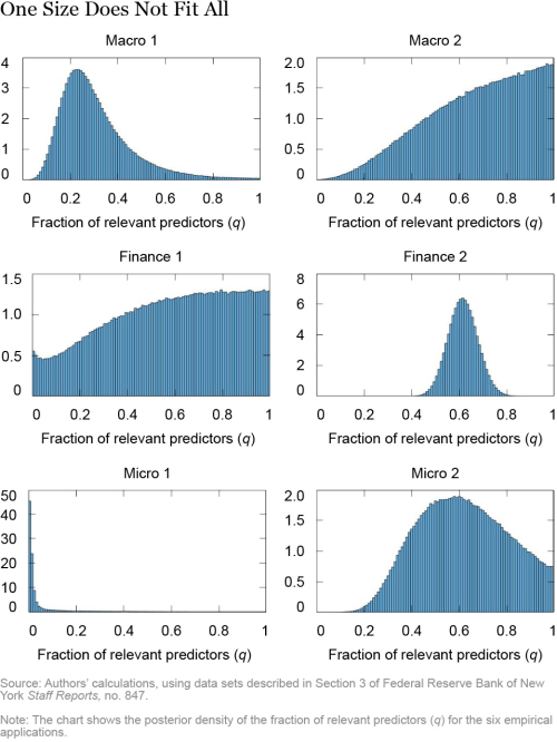
The first key result delivered by our Bayesian inferential procedure is that, in all applications but one, the data do not support sparse model representations. To illustrate this point, the chart below plots the posterior distribution of the fraction of relevant predictors (q) in our six empirical applications. For example, a value of q=0.50 would suggest that 50 percent of the possible regressors should be included. Notice that only in the case of Micro 1 is the distribution of q concentrated around very low values. In all other applications, larger values of q are more likely, suggesting that including more than a handful of predictors is preferable in order to improve forecasting accuracy. For example, in the case of Macro 2 and Finance 1, the preferred specification is the dense model with all predictors (q=1).

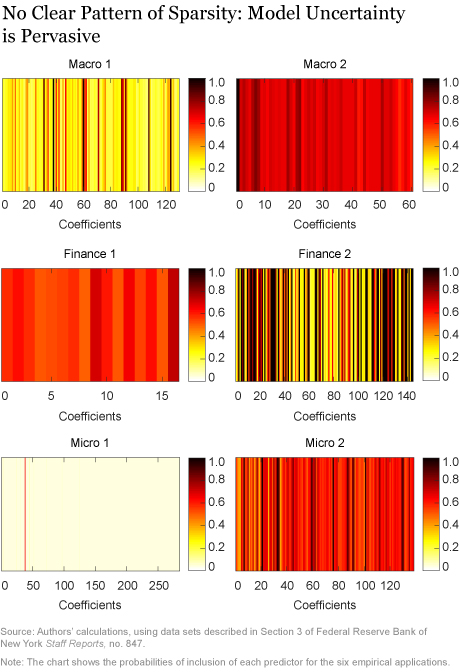
The perhaps more surprising finding is that our results are inconsistent with sparsity even if q is concentrated around values smaller than 1, as in the Macro 1, Finance 2, and Micro 2 cases. To show this point, the chart below plots the posterior probabilities of inclusion of each predictor in the six empirical applications. Each vertical stripe corresponds to a possible predictor, and darker shades denote higher probabilities that the predictor should be included. The most straightforward to interpret is the Micro 1 application. This is a truly sparse model, in which one regressor is selected 65 percent of the time and all other predictors are rarely included.

The remaining five applications do not point to sparsity, in the sense that all predictors seem to be relevant with non-negligible probability. For example, consider the case of Macro 1, in which the best-fitting models are those with q around 0.25, according to the first chart in this post. What the second chart suggests is that there is a lot of uncertainty about which specific group of predictors should be selected, because there are many different models with about 25 percent of the predictors with a very similar predictive accuracy.
Result #2: More Sparsity Only with an A Priori Bias in Favor of Small Models
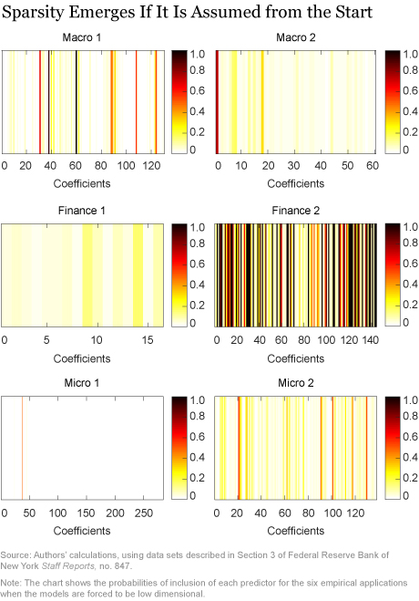
Our second important result is that clearer sparsity patterns only emerge when the researcher has a strong a priori bias in favor of predictive models with a small number of regressors. To demonstrate this point, we re-estimate our model forcing q to be very small. The posterior probabilities of inclusion obtained with this alternative estimation are reported in the chart below. These panels exhibit substantially lighter-color areas than our baseline chart above, indicating that many more coefficients are systematically excluded, and revealing clearer patterns of sparsity in all six applications. Put differently, the data are better at identifying a few powerful predictors when the model is forced to include only very few regressors. When model size is not fixed a priori, model uncertainty is pervasive.

Summing up, strong prior beliefs favoring few predictors appear to be necessary to support sparse representations. As a consequence, the idea that the data are informative enough to identify sparse predictive models might just be an illusion in most cases.
Concluding Remarks
In economics, there is no theoretical argument suggesting that predictive models should include only a handful of predictors. As a consequence, the use of sparse model representations can be justified only when supported by strong statistical evidence. In this post, we evaluate this evidence by studying a variety of predictive problems in macroeconomics, microeconomics, and finance. Our main finding is that economic data do not appear informative enough to uniquely identify the relevant predictors when a large pool of variables is available to the researcher. Put differently, predictive model uncertainty seems too pervasive to be treated as statistically negligible. The right approach to scientific reporting is thus to assess and fully convey this uncertainty, rather than understating it through the use of dogmatic (prior) assumptions favoring sparse models.
Disclaimer
The views expressed in this post are those of the authors and do not necessarily reflect the position of the Federal Reserve Bank of New York or the Federal Reserve System. Any errors or omissions are the responsibility of the authors.

Domenico Giannone is an assistant vice president in the Federal Reserve Bank of New York’s Research and Statistics Group.
Michele Lenza is an economist at the European Central Bank and the European Center for Advanced Research in Economics and Statistics.
Giorgio E. Primiceri is a professor at Northwestern University.
How to cite this blog post:
Domenico Giannone, Michele Lenza, and Giorgio E. Primiceri, “Economic Predictions with Big Data: The Illusion of Sparsity,” Federal Reserve Bank of New York Liberty Street Economics (blog), May 21, 2018, http://libertystreeteconomics.newyorkfed.org/2018/05/economic-predictions-with-big-data-the-illusion-of
-sparsity.html.


 RSS Feed
 Follow Liberty Street Economics