This series examines the Federal Reserve Bank of New York’s dynamic stochastic general equilibrium (FRBNY DSGE) model—a structural model used by Bank researchers to understand the workings of the U.S. economy and provide economic forecasts.
The U.S. economy has been in a gradual but slow recovery. Will the future be more of the same? This post presents the current forecasts from the Federal Reserve Bank of New York’s (FRBNY) DSGE model, described in our earlier “Bird’s Eye View” post, and discusses the driving forces behind the forecasts. Find the code used for estimating the model and producing all the charts in this blog series here. (We should reiterate that these are not the official New York Fed staff forecasts, but only an input to the overall forecasting process at the Bank.)
The model predicts that economic growth will continue to be sluggish as the headwinds from the financial crisis dissipate at a very slow pace. In addition, the negative shocks that have buffeted the economy will continue to restrain investment spending and further slow the recovery. These negative shocks have been offset in the past by expansionary monetary policy, but the positive effects of this policy are set to fade. Because of the still relatively weak economy, inflation remains below the Fed’s long-term objective, with the gap between inflation and the objective closing over the forecast horizon.
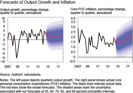
The chart below presents quarterly forecasts for real output growth and the core personal consumption expenditures (PCE) inflation rate over the 2014-17 horizon. These forecasts were generated with data available at the end of July 2014. More specifically, we use data for real GDP growth, core PCE inflation, and the growth in total hours released through the second quarter of 2014, as well as values for the federal funds rate and the spread between BAA corporate bonds and ten-year Treasury yields up to July 30, 2014. The black line represents released data, the red line is the forecast, and the shaded areas mark the uncertainty associated with our forecasts at 50, 60, 70, 80, and 90 percent probability intervals. Notice that the uncertainty around the forecast is minimal for the third quarter of 2014, partly because some of the data used are available for that period of time. Output growth and inflation are expressed in quarter-to-quarter percentage annualized rates.
The model projects a slow recovery with average output growth in the neighborhood of 2 percent throughout the forecast horizon. Moreover, the risks to the forecasts are skewed to the downside: it is more likely that GDP growth will turn out to be below our forecast rather than above. The main reason for this outcome is the zero lower bound on the federal funds rate, which constrains the Fed’s ability to respond appropriately to negative shocks. There is a sizable degree of uncertainty, however, around the real GDP forecast. For example, the model puts at 70 percent the probability that GDP growth (expressed in a Q4/Q4 basis) will be between 1.0 percent and 2.2 percent in the current year, and between -1.3 percent and 4.2 percent in 2015.
Concerning the core PCE inflation forecast, the model predicts an average inflation rate between 1.3 percent and 2.0 percent over the forecast horizon, reaching the long-run Federal Open Market Committee (FOMC) objective of 2 percent only by the end of 2017. Forecast uncertainty is smaller for inflation than it is for output growth. In the near term, the model places high probability on inflation realizations being below the long-run FOMC target, but risks are balanced in the longer term.
Market participants’ expectations about monetary policy are a key determinant of the model’s forecast as they affect the evolution of long-term interest rates. In order to capture the effects of forward guidance, or more generally of the Fed’s communication, the forecast is conditioned on financial market expectations available on July 30, 2014, of the path of the federal funds rate through 2015:Q2. Financial market participants anticipate a federal funds rate liftoff (that is, the first time in which the federal funds rate will be above 25 basis points) as happening in 2015:Q2. (Our working paper provides more details about the implementation of forward guidance in the model.) After the second quarter of 2015, we let the model set the path of the policy rate according to the “historical” interest rate rule, the one that we estimated over the pre-zero-lower-bound period. Of course, monetary policy might end up behaving differently from what is suggested by the estimated historical rule, but historical behavior is a reasonable starting point for a forecast. Under the current forecast, the model predicts the federal funds rate to return very slowly to its long-run level.
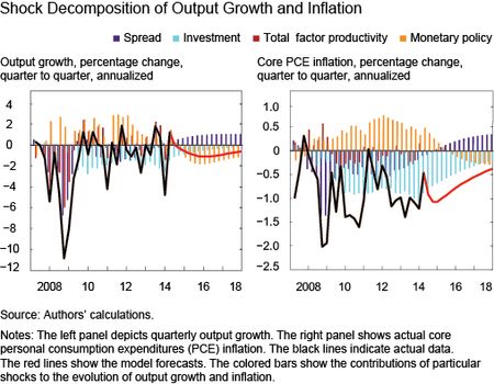
As explained in the third post in this series, the model provides a narrative of the driving forces behind economic events, using the “shock decomposition” technique. The next chart shows that U.S. economic performance since the Great Recession has been driven primarily by two factors: headwinds hindering aggregate demand and monetary stimulus. Tight credit (in purple) and other factors restraining investment demand (in light blue) abated only very gradually, contributing to a holding back of the economy during the recovery. The persistent slack in the economy results in a rate of inflation coming in below the Fed’s long-run target. Looking ahead, the negative effect of the credit shocks (in purple) that generated the Great Recession are expected to wane. In fact, these shocks start to support growth starting in early 2014, consistent with the significant reduction in perceived risks and the ensuing compression in credit spreads observed recently. However, after the recession the economy has continued to be buffeted by negative shocks restraining investment (in light blue). The cumulative impact of these shocks on the level of output has not yet reached its full brunt, and consequently they still exert a negative impact on growth.
These negative shocks have been offset by expansionary monetary policy. In particular, forward guidance about the future path of the federal funds rate has played an important role in counteracting headwinds and has lifted output and inflation. The orange bars in the chart above show that the cumulative impact of policy accommodation, as measured by the current level of the federal funds rate in deviation from what is implied by the estimated historical rule. Through the first half of 2014, monetary policy provided substantial policy stimulus to the output growth. However, the positive effect of this policy accommodation on the level of output begins to wane at the end of 2014 and onward, as illustrated by the negative contribution of monetary shocks to output growth, even though it continues to maintain the policy rate lower than it would otherwise be. Why is that? In the model, monetary policy has no real effects in the long run, consistent with a long tradition in macroeconomics dating back to the so-called expectations-augmented Phillips curve of Friedman and Phelps. Therefore, monetary policy shocks can only have temporary effects on the level of output. If they push output up today, providing a positive contribution to its growth rate, then sooner or later that positive contribution must be reversed, so that output can ultimately return to its original level.
Note that the chart shows only the most important shocks that have buffeted the U.S. economy in recent years. The chart omits in particular price markup shocks which capture short-term movements in inflation, such as those due to changes in commodity prices. Over the past few years, these shocks have driven some of the fluctuations in inflation, especially during the Arab Spring crisis (as discussed in yesterday’s post, “An Assessment of the FRBNY DGSE Model’s Real-Time Forecasts, 2010-13”). However, in this model, the impact of these shocks is short-lived and hence does not affect the medium- and long-term movements in inflation. (See this paper for an in-depth discussion of this issue.)
In conclusion, the FRBNY DSGE model, at this point, predicts a continued gradual recovery in economic activity with a progressive return of inflation toward the FOMC’s long-run target of 2 percent, as the negative effect of the Great Recession continues to dissipate. This forecast remains surrounded by significant uncertainty, with the risks slightly skewed to the downside for output growth because of the constraint on policy imposed by the zero lower bound.
Disclaimer
The views expressed in this post are those of the authors and do not necessarily reflect the position of the Federal Reserve Bank of New York or the Federal Reserve System. Any errors or omissions are the responsibility of the authors.
Matthew Cocci is a senior research analyst in the Federal Reserve Bank of New York’s Research and Statistics Group.
Marco Del Negro is an assistant vice president in the Group.
Stefano Eusepi is a research officer in the Group.
Marc Giannoni is an assistant vice president in the Group.
Sara Shahanaghi is a research analyst in the Group.


 RSS Feed
 Follow Liberty Street Economics
Thank you for the question. Our publishing of this blog series and, in particular, our release of the code provides the best opportunity for the public to examine the code and test its properties. We work to validate our models, both in the narrow sense of testing the accuracy of the code, and in the broader sense of testing and judging its accuracy and usefulness as an economic model. Our record of publication and peer review is aimed precisely at this public examination. One informal approach of testing a model’s usefulness is to simply look at past forecasts and compare them with actual outcomes, which is what we did in Friday’s post, “An Assessment of the FRBNY DSGE Model’s Real-Time Forecasts, 2010-13.” By this informal metric, our model appears to be relatively successful.
As someone now supervised by the Fed, can you tell me whether the model has undergone a formal Model Validation?
Great job on releasing this to the public! I would just like to point out, in the name of open science, that while the code for these forecasts in written in MATLAB, in all likelihood it will also run on Octave, which is an open-source language that is mostly compatible with MATLAB.