The current policy debate is influenced by the possibility that the first-quarter GDP data were affected by “residual seasonality.” That is, the statistical procedures used by the Bureau of Economic Analysis (BEA) did not fully smooth out seasonal variation in economic activity. If this is indeed the case, then the weak readings of the economy in the first quarter give an inaccurate picture of the state of the economy. In this post, we argue that unusually adverse winter weather, rather than imperfect seasonal adjustment by the BEA, was an important factor behind the weak first-quarter GDP data.
Recent studies by economists at the Federal Reserve Bank of San Francisco as well as a number of private sector research firms (as summarized by the Wall Street Journal) suggest that there are problems with the seasonal adjustment of GDP data for the first quarter of the year. A study by economists at the Board of Governors of the Federal Reserve, however, did not find significant statistical evidence for such distortions on the aggregate GDP level, although they found weak evidence for some of its components.
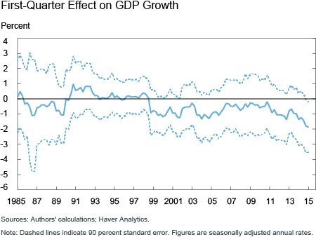
We revisit the issue of residual seasonality using regression analysis. As a start, seasonally adjusted annualized GDP growth is regressed on a constant, seasonal dummies for each of the first, second, and fourth quarters, and lagged GDP growth rates, using data from 1975 through the first quarter of 2015. The hypothesis is that an accurate seasonal adjustment would make the seasonal dummies statistically insignificant, whereas a significant seasonal dummy suggests an unexplained influence on growth rates in certain quarters even after seasonal adjustment. Regressions are estimated using moving ten-year data windows. The chart below shows the evolving estimates of the first-quarter seasonal dummy parameter over our sample. The coefficient estimates are not statistically significant until the final estimation window, which finds uncorrected seasonality in the first quarter over the past ten years, averaging almost 2 percentage points in annualized terms. The seasonal dummies for the second and fourth quarters are never significantly different from zero.

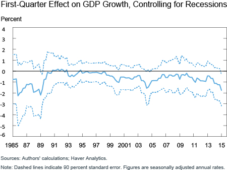
Using sliding ten-year windows of data means some of the regressions will be dominated by recessions. To correct for this effect, we add an NBER recession dummy variable and repeat the analysis, the results of which are shown in the chart below. The results are essentially the same.

The next round of analysis is to see if the recent negative first-quarter readings might be the result of harsher-than-usual winter weather. To make this assessment, we use a mixed-frequency regression for GDP growth with monthly variables that measure how much the temperature undershoots relative to the monthly average in both the current and previous quarters plus lagged quarterly growth rates. Using monthly temperature data allows the model to let weather in some months be more important than in others. This model’s out-of-sample forecasting ability of GDP growth is better than a more basic model with only lagged growth rates and a constant, suggesting that data on adverse weather conditions are useful information in tracking GDP growth.
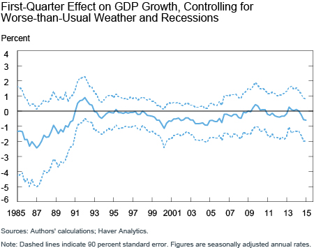
Given this outcome, we repeated the above analysis for residual seasonality with a new variable that proxies the growth impact of weather severity in the current quarter using our weather conditions data. The final chart below depicts how the potential growth impact of residual seasonality in the first quarter evolved over our sample. The estimated impact is now much more centered toward zero and it never becomes statistically significant now that the impact of adverse weather is accounted for separately in the regression. As for the likely weather impact on GDP growth, the model has the unusually cold readings for the first quarter of 2015 taking about 2 percentage points off growth on an annualized basis.

It will not be surprising if the question of residual seasonality comes up again next year when first-quarter growth numbers are announced. This analysis highlights that the usefulness of seasonally adjusting data can be hampered by weather conditions that are unusual relative to the period over which the seasonal factors were calculated.
Disclaimer
The views expressed in this post are those of the authors and do not necessarily reflect the position of the Federal Reserve Bank of New York or the Federal Reserve System. Any errors or omissions are the responsibility of the authors.

Jan J.J. Groen is an officer in the Federal Reserve Bank of New York’s Research and Statistics Group.
 Patrick Russo is a senior research analyst in the Bank’s Research and Statistics Group.


 RSS Feed
 Follow Liberty Street Economics
Mohit— You are correct that each of the dummy variables for Q1, Q2, and Q4 are equal to either 0 or 1. Also in the regression, we have a constant (which is always equal to 1), (sometimes) the lagged quarterly growth rate, the recession dummy, and the estimated weather contribution. So for the equation estimating 2015Q1 growth, Q1 is equal to 1 (and Q2 and Q4 are equal to 0), the recession dummy is equal to 0, and the constant is equal to 1, as always. The lagged growth rate for 2015Q1 would be the growth rate from 2014Q4, which was 2.2 percent. With this set-up, the coefficient on Q1, is the average difference between Q1 growth and Q3 growth (after taking account of recessions, lagged growth, and weather).
I was having some difficulty as to how the analysis was structured using the regression approach to capture the effect of various quarters using “constant dummy variables” . As per my understanding, the dummies for Q1, Q2 and Q4 would have been used and put as 1 or 0 and the lagged GDP growth would be the quarterly growth. Could someone please help me understand this with the help of an example.