How Large Are Default Spillovers in the U.S. Financial System?

Fernando M. Duarte, Collin Jones, and Francisco Ruela

When a financial firm suffers sufficiently high losses, it might default on its counterparties, who may in turn become unable to pay their own creditors, and so on. This “domino” or “cascade” effect can quickly propagate through the financial system, creating undesirable spillovers and unnecessary defaults. In this post, we use the framework that we discussed in “Assessing Contagion Risk in a Financial Network,” the first part of this two-part series, to answer the question: How vulnerable is the U.S. financial system to default spillovers?

Detailed Network Data is Difficult to Obtain

The main challenge in estimating the expected value of default spillovers is that it requires knowledge of all the bilateral claims between each pair of nodes. Such granularity of data is not publicly available. Moreover, for some financial firms in less regulated parts of the financial system, such data may not even exist, except in fragmented form inside the firms themselves.

One way out of this limitation is to fill in the data gaps with artificial data simulated from a model. Another way is to construct top-down measures of interconnectedness that rely on more readily available data, such as stock market returns, instead of actual network-specific data. However, this also requires a model to tie the non-network specific data to the default spillovers we are trying to measure. A third strategy is to narrow down the network of interest enough—say, to a single asset or narrow subsector— so that all bilateral exposures can be obtained.

An Upper Bound on Network Default Spillovers

Our goal is to estimate expected default spillovers for the entire U.S. financial network, across all institutions and asset classes, with the fewest assumptions possible. To do so, we use a new way to deal with the problem of data deficiency proposed by Glasserman and Young. They show that for a very broad class of models, even though the actual expected spillover losses cannot be computed without knowledge of all bilateral exposures, an upper limit to these spillovers can be estimated using only node-specific information (that is, without a precise breakdown of the nodes’ counterparties or the magnitudes of obligations to them). In particular, the upper limit is based on each node’s probability of default, its total outside assets, and its ratio of inside liabilities to total liabilities. Thus, at the cost of estimating an upper bound on spillovers instead of their actual values, the data requirements are greatly reduced.

The upper bound shows how much larger expected losses in the connected network are, when compared to expected losses in an analogous disconnected network with its interconnections removed (see part 1 of this series for details). Estimating the upper bound in this way enables us to quantify the effects of the network structure, without needing additional assumptions about the initial shocks to each node’s outside assets.

Having an upper limit is very useful, especially if it turns out to be low. Indeed, if we know that the maximum possible expected default spillovers are negligible, then there is little gain in estimating the actual quantity.

Empirical Estimate

With this less stringent data requirement, in a New York Fed Staff Report, we study a network that captures around 85 percent of all assets of the U.S. financial system as reported in the Financial Accounts of the United States. We use publicly available data together with commercially available data from Moody’s. The chart below shows the upper limit on expected losses due to network default spillovers as a percentage of expected losses in the analogous disconnected network. In other words, the line in the chart shows an upper bound on the losses that can be attributed to the default spillovers as a fraction of the initial direct losses that do not stem from network effects.

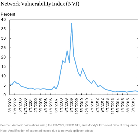
The chart shows that between 2002 and 2007, the upper bound on default spillovers is rather small, which means that the financial network is robust to contagion arising from counterparty risk. However, between 2008 and 2011, the upper bound on spillovers is meaningfully above zero. Our results suggest that the financial network is most fragile in the first quarter of 2009, when we estimate that network default spillovers can amplify initial losses by up to 40 percent. After that quarter, the upper bound on default spillovers starts to decline and reverts to pre-crisis levels by 2015.

Individual Node Behavior

To understand how individual firms are influenced by and affect the network spillovers, we define the “financial connectivity” of a firm to be the fraction ratio of a firm’s inside liabilities to total liabilities. A firm specific “contagion index” can then be computed by multiplying the firm’s financial connectivity, its net worth, and the leverage of its outside assets (calculated as outside assets divided by net worth). The contagion index gives the worst-case payment shortfall that a firm can pass on to other nodes of the network. The table below shows the firms with the highest contagion index for the last quarter of 2016 together with their financial connectivity, outside assets and net worth.

The first notable feature of the table is that it is almost exclusively populated by bank holding companies, even though our sample contains insurance companies, asset managers, and many other types of financial institutions. In addition, the banks are fairly different with respect to why their contagion index is high. For example, the node with the largest connectivity is the one labeled “Top 10 Dealers,” which is a single node that aggregates the largest ten broker-dealers (we do not show individual results for broker-dealers for confidentiality reasons). Compared to the four nodes with the highest contagion index, the top 10 dealer node has a higher connectivity but lower outside assets.

Digging Deeper

Estimating an upper bound on spillovers is most useful when its value turns out to be low, since then we can then be more confident that actual spillovers are expected to be low. When the upper bound is high, as in 2008-09, actual expected spillovers can be as high as the bound or as low as zero. One way to obtain some further insight into situations in which the estimated upper bound is relatively high and uninformative is to look at all possible network topologies that are consistent with the observed data.

In the illustration below we show, for the third quarter of 2008, two possible network configurations for a subset of nodes. The size of the nodes represents their net worth, and the thickness of the connections represents the size of obligations between two nodes. The network on the left was constructed by looking at the set of all possible bilateral positions among nodes that yield the same node-specific numbers that we observe in the data, and then picking the bilateral positions that produce the largest expected default spillovers. The network on the right was found analogously by minimizing, rather than maximizing, the default spillovers. The most benign configuration has spillovers that are an order of magnitude lower than the “worst case” network, highlighting the importance of network topology.

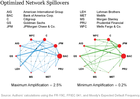
Both worst-case and best-case networks show large bank holding companies, broker-dealers, and AIG being highly interconnected. However, the worst-case network has more connections, with AIG, JPMorgan Chase, and especially Lehman Brothers, having a large exposure to Citibank. The two networks thus illuminate how the failure of a single firm such as Lehman Brothers could have vastly different default spillover effects depending on the particular firms with which it is connected.

Fernando M. Duarte is an economist in the Federal Reserve Bank of New York’s Research and Statistics Group.

Collin Jones is a former senior research analyst in the Bank’s Research and Statistics Group and a Ph.D. student in economics at University of California, Berkeley.

Francisco Ruela is a senior research analyst in the Bank’s Research and Statistics Group.

How to cite this post:

Fernando M. Duarte, Collin Jones, and Francisco Ruela, “How Large are Default Spillovers in the U.S. Financial System?,” Federal Reserve Bank of New York Liberty Street Economics, June 26, 2019, https://libertystreeteconomics.newyorkfed.org/2019/06/assessing-contagion-risk-in-a-financial-network.html.

---

Disclaimer

The views expressed in this post are those of the authors and do not necessarily reflect the position of the Federal Reserve Bank of New York or the Federal Reserve System. Any errors or omissions are the responsibility of the authors.