On the Distributional Consequences of Responding Aggressively to Inflation

Marco Del Negro, Keshav Dogra, Pranay Gundam, Donggyu Lee, and Brian Pacula

This post discusses the distributional consequences of an aggressive policy response to inflation using a Heterogeneous Agent New Keynesian (HANK) model. We find that, when facing demand shocks, stabilizing inflation and real activity go hand in hand, with very large benefits for households at the bottom of the wealth distribution. The converse is true however when facing supply shocks: stabilizing inflation makes real outcomes more volatile, especially for poorer households. We conclude that distributional considerations make it much more important for policy to take into account the tradeoffs between stabilizing inflation and economic activity. This is because the optimal policy response depends very strongly on whether these tradeoffs are present (that is, when the economy is facing supply shocks) or absent (when the economy is facing demand shocks).  

Demand Shocks 

In this post, we want to understand how the volatility of aggregate and distributional variables (that is, for instance, consumption of the poorest 10 percent of the population) changes depending on the reaction function of the monetary authorities. Given that the U.S. economy has been experiencing an inflationary episode, we focus in particular on the Fed’s response to inflation and ask how volatility changes as the monetary authorities respond more aggressively to inflation. We study the effects on volatility because higher volatility means higher economic uncertainty for households, which generally translates into lower welfare (although this is not necessarily always the case, as discussed later).  

For reasons that will soon be apparent, it is helpful to identify the different sources of volatility in answering this question. In particular, it is helpful to distinguish so-called demand disturbances—that is, shocks that push output and inflation in the same direction—from supply disturbances, which push them in the opposite direction and create a tradeoff for the central bank. Examples of the former are shocks arising from the financial sector: in the aftermath of the great financial crisis for instance the economy was depressed and inflation was for a long period below the Fed’s target. Examples of the latter are cost-push shocks such as those studied in our companion post. 

We first look at so-called demand shocks. The model we use (Lee, 2024) features a number of these shocks, including a shock to financial institutions’ investment preferences (risk premium shocks), a shock to households’ discount factor (discount factor shocks), and a shock to transfers from the government to individuals (transfer shocks), such as those witnessed in the aftermath of the pandemic. 

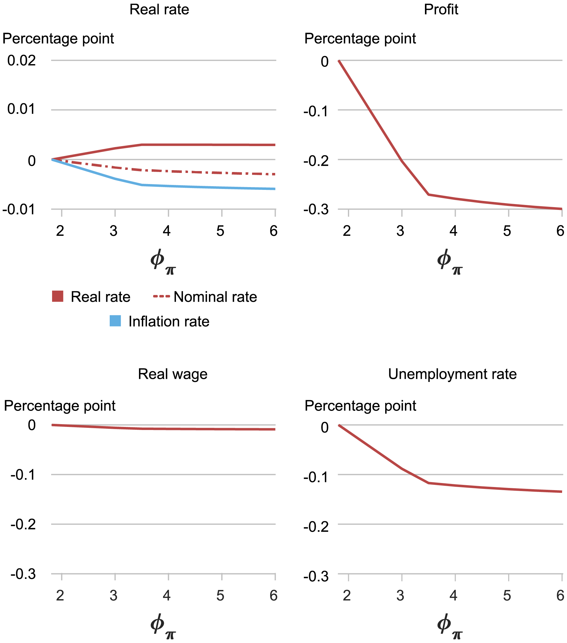
The chart below shows how the standard deviations of real and nominal rates, inflation, real wages, profits, and unemployment change as we increase the coefficient on inflation in our Taylor-like interest-feedback rule starting at its estimated baseline value of 1.8. Specifically, the chart depicts percentage point changes in the standard deviation of each variable relative to the baseline. In this exercise, we assume that the economy is subject only to demand shocks. The chart shows that a more aggressive response to inflation reduces the volatility not only of inflation, which is obviously to be expected, but also of all aggregate variables except real rates. This result is akin to the so-called “divine coincidence” in the textbook New Keynesian model (even though this coincidence does not hold exactly in HANK models): taming inflation is tantamount to taming the real effects of the shocks driving inflation. In other words, nominal and real stabilization go hand in hand when the economy is faced with demand shocks.  

Volatility of Aggregate Variables as Policy Responds More Aggressively to Demand Shocks  

The next chart looks at the distributional implications of changing the response to inflation. It shows the volatility of consumption for households in different parts of the wealth distribution (specifically, we report the average change in standard deviation for households in the top and bottom 10 percent of the wealth distribution, the middle 20 percent, and all households).  

Volatility of Consumption by Wealth as Policy Responds More Aggressively to Demand Shocks  

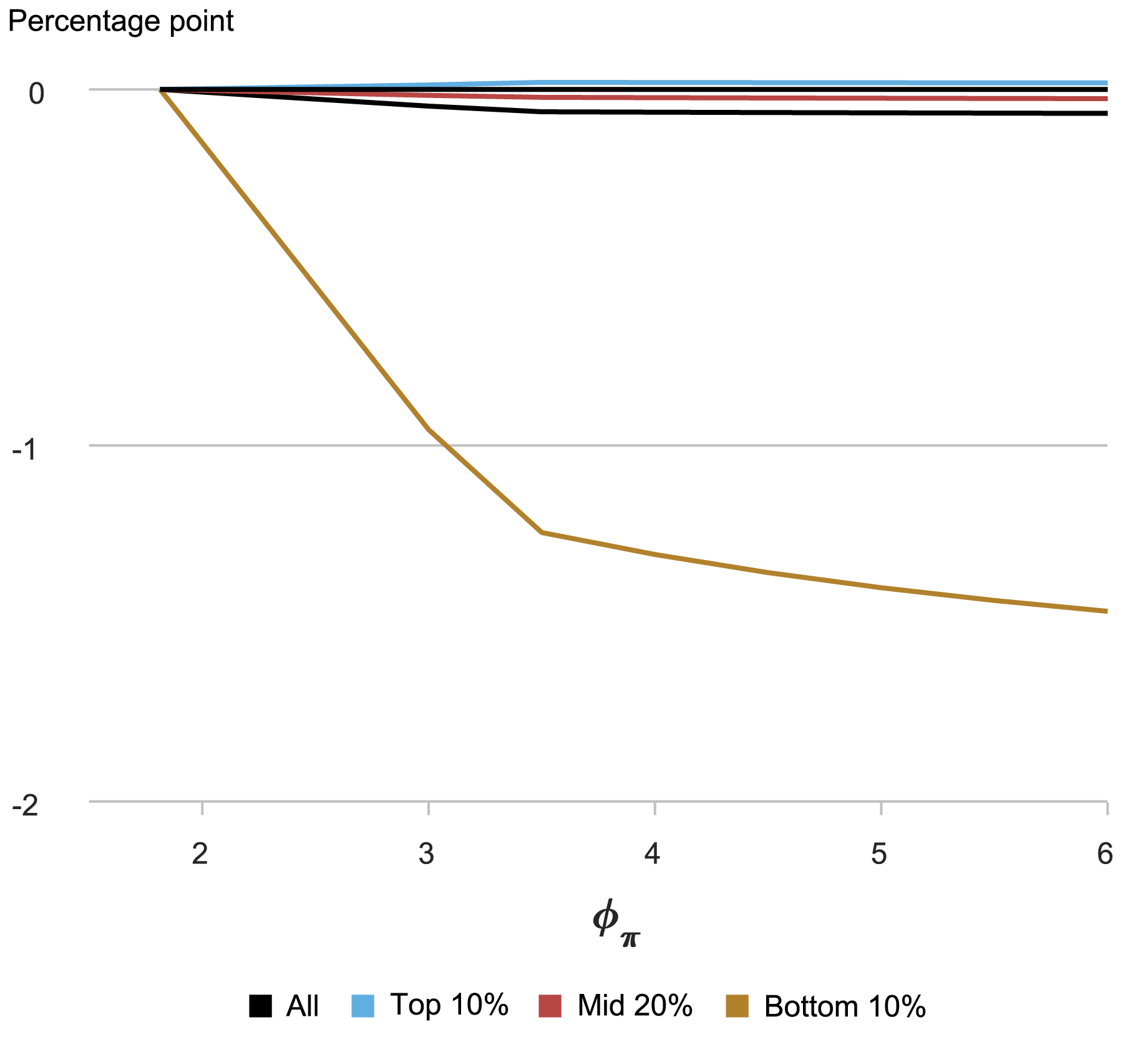
The chart shows that consumption volatility generally declines when the response to inflation is more aggressive. Again, the divine coincidence provides intuition for this result: responding to inflation is tantamount to offsetting the effects of the shock on economic activity. Since these are the sources of consumption volatility, offsetting the shock leads to lower volatility. The chart also shows that the reduction in volatility associated with a stronger response to inflation is particularly striking for households at the bottom of the wealth distribution. This is the case because poor households are more vulnerable to shocks, as they have no wealth that enables them to smooth out the consequences of shocks over time (in fact, many of them are in debt). Wealthier households can use their savings buffer to maintain their living standards even in the face of economic adversities. Households who have reached their debt limit, or are close to it, cannot and are, quite literally, hand-to-mouth. In fact, even households with some wealth may also be effectively hand-to-mouth to the extent that their wealth is illiquid (for example, housing or pension plans), because trying to use this wealth to buffer shocks is costly.  

Supply Shocks

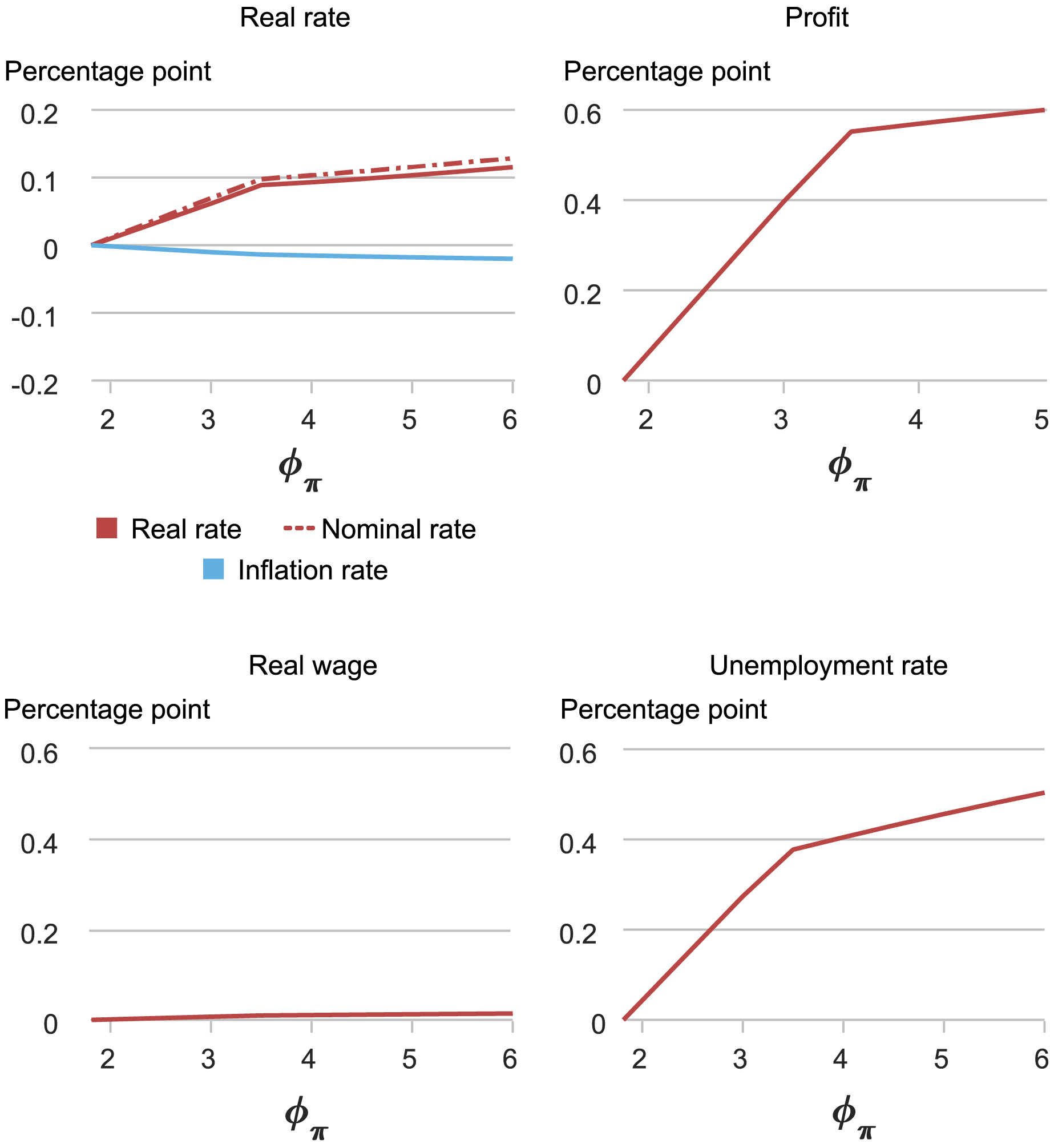
The next two charts show how volatility changes for both aggregate and distributional variables when only supply shocks, like those considered in our companion post, are present. Clearly, the picture is very different. Inflation volatility still declines as the monetary authority responds more aggressively to inflation, but the divine coincidence no longer applies: both aggregate and distributional variables become more volatile as policy responds more aggressively to inflation. This is because supply shocks push real activity and inflation in opposite directions: policymakers can only stabilize inflation at the cost of forcing output and employment farther away from steady state. For instance, an adverse cost-push shock causes higher inflation and lower output. The higher inflation can only be fought by raising interest rates and pushing output further down.

Volatility of Aggregate Variables as Policy Responds More Aggressively to Supply Shocks 

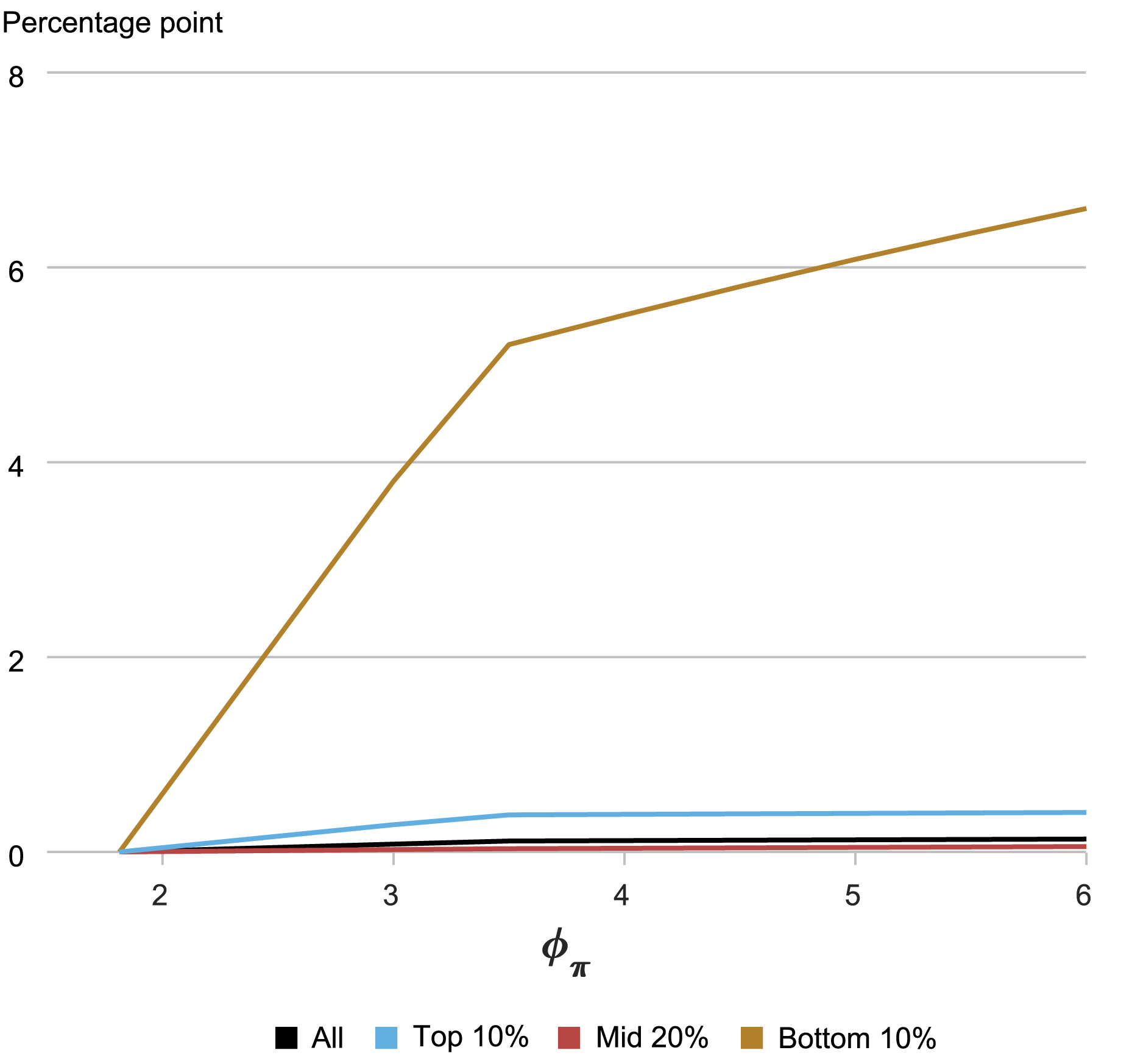
In sum, supply shocks generate a tradeoff for the central bank between stabilizing inflation and real activity, so that a stronger response to inflation results in higher instability of the real economy. This instability is particularly harmful for households in the bottom 10 percent of the wealth distribution, as shown in the chart below. In the HANK model with sticky nominal wages these households are particularly hurt by inflation volatility because this translates into fluctuations in their real wages. If these households are hand-to-mouth, fluctuations in the real wage translate one-to-one into consumption volatility. In spite of this, the additional volatility in real activity generated by a more aggressive response to inflation hurts poor households even more according to the model, as we have seen in our companion post.   

Volatility of Consumption by Wealth as Policy Responds More Aggressively to Supply Shocks 

Implications for Policy

Deriving the policy implications of these results is no trivial task for a number of reasons. First, we do not know what disturbances the future will bring. After many years in which demand-type shocks like the financial crisis seemed to be dominant, the world just experienced an inflationary episode in which cost-push shocks arguably played an important role. Second, higher/lower volatility does not always translate into lower/higher welfare. For example, it would not be optimal to fully stabilize consumption in response to productivity shocks, as those shocks lead to fluctuations in the efficient levels of output that should be accommodated. Directly calculating the effect of alternative policies on household welfare, however, would require approximating our model up to second order, which is technically challenging in HANK models (Bhandari et al. 2023 describe one approach to perform this approximation; Acharya et al. 2023 study optimal policy in a tractable HANK model which can be solved up to second order in closed form.).  

That being said, our results are broadly in line with some of the growing literature on optimal policy in HANK models. It is well known that in simple New Keynesian representative agent models Taylor-type feedback rules are not optimal. In these models the optimal policy is best described as a form of ”flexible price-level targeting,” in which policy puts some weight on stabilizing both the price level and the output gap (see Svensson and Woodford, 2004). Acharya et al. find that a similar policy can be optimal in HANK economies, provided that it puts some weight on stabilizing the level of output, not just the output gap, and puts less weight on stabilizing prices than would be optimal in a representative agent New Keynesian model. If a disturbance would tend to push inflation and the output gap on the same side of the dual mandate—for example, a negative demand shock which reduces both inflation and output—optimal policy calls for aggressively adjusting interest rates to quash the effects of the shock and fully stabilize both variables. But if the disturbances cause inflation and the output gap to be on the opposite side of the dual mandate, as is the case with cost-push shocks, optimal policy calls for a less aggressive response, given the tradeoff between stabilizing inflation and economic activity. Taking into account the distributional implications of monetary policy—as we have done in these posts—suggests that accounting for the tradeoff between inflation and economic activity is even more important than when these distributional consequences are ignored. 

How to cite this post:
Marco Del Negro, Keshav Dogra, Pranay Gundam, Donggyu Lee, and Brian Pacula, “On the Distributional Consequences of Responding Aggressively to Inflation,” Federal Reserve Bank of New York Liberty Street Economics, July 3, 2024, https://libertystreeteconomics.newyorkfed.org/2024/07/on-the-distributional-consequences-of-responding-aggressively-to-inflation/.