Differences in Rent Inflation by Cost of Housing

Jonathan McCarthy and Richard Peach

Update (12.9.15): We revised the chart package linked to in the second paragraph of this post to correct a spreadsheet error. A new note also clarifies our methodology. Please see the addendum below.

We know that different people experience different inflation rates because the bundle of goods and services that they consume is different from that of the “typical” household. This phenomenon is discussed in this publication from the Bureau of Labor Statistics (BLS), and this article from the New York Fed. But did you know that there are substantial differences in inflation experience depending on the level of one’s housing costs? In this post, which is based upon our updated staff report on “The Measurement of Rent Inflation,” we present evidence that price changes for rent, which comprises a large share of consumer spending, can vary considerably across households. In particular, we show that rent inflation is consistently higher for lower-cost housing units than it is for higher-cost units. Note that since owners’ equivalent rent inflation is estimated from observed changes in rent of rental units, this finding applies to homeowners as well. While we cannot be certain about why this is the case, it appears to be at least partly related to how additional units are supplied to the housing market: in higher-price segments additional units primarily come from new construction, while most of the increase in lower-price segments comes from units that previously were occupied by higher-income households.

In our staff report, we derive estimates of tenant rent inflation and owners’ equivalent rent inflation using data from the American Housing Survey (AHS) national sample for years 1989 through 2013 (this survey is conducted in odd numbered years). We follow the BLS methodology as closely as possible for estimating these two inflation rates. While our estimates are on average somewhat higher than those published by the BLS, the differences generally are not statistically significant (see Table 4 in the chart package of our staff report).

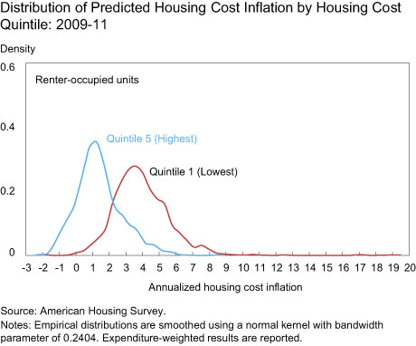
In deriving our rent inflation estimates, we estimate a panel regression of the change in housing cost (rent plus utilities) of individual rental units. Consistent with BLS’s findings, we find that the log level of housing cost and geographic location are the primary determinants of the change in rent. Interestingly, the estimated coefficient on the log of housing cost in this regression is negative and highly significant. We illustrate this inverse relationship in the chart below, which presents the distributions of housing cost inflation over 2009-11 for rental units whose cost in 2009 was in the lowest quintile (20 percent) of housing costs and for rental units in the highest-cost quintile (the distributions for the other quintiles are shown in chart package of our staff report). The distribution for the highest quintile lies to the left of that for the lowest quintile, indicating that housing cost inflation of more expensive units generally was below that of lower cost units.

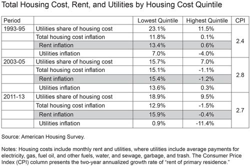
What is behind this inverse relationship? We explore two potential explanations. One possibility is that utilities comprise a higher share of housing cost for lower-cost units and that, on average, utilities prices increase faster than rent. The table below sheds light on this possibility, showing total housing cost inflation, rent inflation, and utility cost inflation for the highest and lowest housing cost level quintiles in some selected periods. While it is true that utilities represent a higher share of total housing cost for the lowest quintile, even when one looks at rent inflation alone, it remains the case that it is lower for the highest housing cost quintile than it is for the lowest quintile.

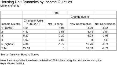
The second possibility we examine is the sources of new housing supply across the housing cost distribution. To do this, we divide the 1989 AHS sample into quintiles based on the reported household income associated with each housing unit (quintile 1 is the lowest-income quintile, while 5 is the highest). We use income rather than housing cost because in the AHS owner-occupied housing units are not assigned a housing cost that is conceptually equivalent to that which is assigned to rental units. We then go to the 1991 AHS sample and divide it into income quintiles based on 1991 income deflated (using the personal consumption expenditures deflator) to 1989 dollars. We then determine the change in the number of occupied units over 1989-91 and the sources of that change: those sources include new construction, filtering from one income quintile to another, and what we call net conversions of units to or from residential usage [this includes units lost in situations like demolition or fire and units gained by conversion from nonresidential uses or by subdividing a single unit]. We then repeat the exercise for 1991 to 1993, and so on, and compute a running total of the change in units by source for each income quintile.

In determining whether a unit has filtered into a different income quintile, we impose the following requirement: If there is a change in the household income associated with a unit that is sufficient to place it in a different income quintile from that of the base year, the occupants in the second year of the panel must have moved into the unit after the survey date of the base year. With this requirement, we rule out from our definition of filtering income shocks for a given household due to events such as changing to a better job, retirement, or the loss of an earner in cases such as death, divorce, or illness.

The results from this exercise are presented in the table below. According to our estimates, 32.3 million occupied units were added through new construction between 1989 and 2013, which is close to data on housing completions published by the U.S. Census Bureau (31.6 million units). For the highest-income quintile, new construction (10.8 million units) is about 2½ times the net increase in housing units (4.3 million units). As one moves down the income distribution, new construction represents a declining share of the net increase in housing units. At the lowest-income quintile, new construction (3.1 million units) is only about two-thirds of the net increase (4.5 million units). Consequently, filtering and net conversions are of increasing significance as sources of the net increase of housing units as one moves down the income distribution.

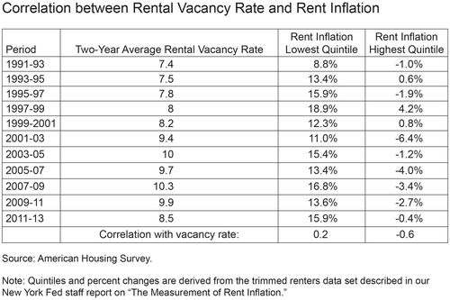
Additional evidence of the varying degree to which newly constructed housing units influence rent inflation is presented in the last table. The first column shows two-year average rental vacancy rates from the Census Bureau. The next two columns shows annualized two-year rent changes for the lowest and highest housing cost quintiles. The bottom of the table displays the correlation coefficient between the rental vacancy rate and the rent changes in each quintile. In the highest quintile, there is a sizable negative correlation between the rental vacancy rate and rent inflation; that is, lower vacancy rates are associated with higher rent inflation and vice versa. Thus, higher rent inflation in the highest housing cost quintile provides an incentive for new construction, which, in turn, dampens future rent increases. Conversely, for the lowest housing cost quintile, the correlation is small and positive, indicating that rent inflation is less influenced by fluctuations in the volume of new supply.

Putting these various threads together, it appears that the inverse relationship between prior rent levels and rent inflation may be related to a greater concentration of new residential construction in the higher rent level segments of the housing market, dampening the price response to a tightening in that market.  As one moves down the rent level distribut
ion, increases in the supply of housing increasingly come from previously higher-rent units, which may still have rents above the average of the incumbent units, pushing up rents more in such segments.

One interesting question is how various public policies designed to influence the level of housing costs affect the growth of that cost over time. We hope to explore this issue in future work.

Addendum

Our analysis of rent inflation is based on data panels that span three American Housing Surveys (AHS). For example, to estimate rent inflation over the years 2011 to 2013, we confine our analysis to rental units for which we have complete observations from the 2009, 2011, and 2013 surveys. In our model, housing cost change from 2011 to 2013 is regressed on the log level of housing cost in 2009 plus several variables pertaining to the location and physical characteristics of the unit. In the tables in which we present information by housing cost quintiles, the quintiles are based on housing cost levels of 2009.

Our finding that housing cost inflation is inversely related to the level of housing cost holds in each panel. However, that result does not necessarily hold when comparing rent levels across panels, particularly as the time span between panels increases. This fact does not negate our finding as each panel is a separate sample. The greater the time span between panels, the greater the likelihood that the sample of rental units analyzed has changed.

Disclaimer
The views expressed in this post are those of the authors and do not necessarily reflect the position of the Federal Reserve Bank of New York or the Federal Reserve System. Any errors or omissions are the responsibility of the authors.

---

Jonathan McCarthy is a vice president in the Federal Reserve Bank of New York’s Research and Statistics Group.

Richard Peach is a senior vice president in the Bank’s Research and Statistics Group.