As central banks shrink their balance sheets to restore price stability and phase out expansionary programs, gauging the ampleness of reserves has become a central topic to policymakers and academics alike. The reason is that the ampleness of reserves informs when to slow and then stop quantitative tightening (QT). The Federal Reserve, for example, implements monetary policy in a regime of ample reserves, whereby the quantity of reserves in the banking system needs to be large enough such that everyday changes in reserves do not cause large variations in short-term rates. The goal is therefore to implement QT while ensuring that reserves remain sufficiently ample. In this post, we review how to gauge the ampleness of reserves using the new Reserve Demand Elasticity (RDE) measure, which will be published monthly on the public website of the Federal Reserve Bank of New York as a standalone product.
In a Liberty Street Economics post in 2022, we proposed focusing on the slope of the reserve demand curve to assess the ampleness of reserves in the banking system. The reserve demand curve describes the price at which banks are willing to trade their reserve balances with one another as a function of aggregate reserves. In the U.S., this price is called the federal funds rate, which is the rate targeted by the Federal Open Market Committee (FOMC) in its communication of the monetary policy stance. The slope of the reserve demand curve measures the elasticity of the federal funds rate to changes in the level of reserves; that is, by how much this rate changes in response to variation in aggregate reserves. We call this quantity the Reserve Demand Elasticity.
Economic theory tells us that the RDE (that is, the slope of the reserve demand curve) is different at different reserve levels. We can then operationalize the notion of ample reserves in the Federal Reserve monetary policy framework as the region of the reserve demand curve where the slope is only modestly negative: for this range of reserve levels, the RDE is small. At higher reserve levels, where reserves in the banking system are abundant, the RDE is zero (the demand curve is flat); at lower levels, where reserves are scarce, the RDE is negative and large (the curve is steeply sloped). To operate in an ample reserves framework and avoid reserve scarcity, it is therefore important to identify the transition point between abundant and ample reserves.
Identifying the transition between these regions is challenging because banks’ demand for reserves fluctuates over time and, in turn, the supply of reserves may respond to sudden changes in banks’ demand. As explained in our paper, we developed an econometric methodology that addresses these challenges. The idea is simple: exploiting large fluctuations in aggregate reserves over the last decade, we move along the reserve demand curve and, for each day, estimate its slope (the RDE).
In the first post of a two-part Liberty Street Economics series published this summer, we propose building on our methodology to monitor reserve ampleness in real time. We estimate the RDE daily using only information available as of each day, making our estimates equivalent to real-time calculations. We can then construct a signal of ampleness of reserves by looking at when the real-time estimates of the RDE become negative at a given confidence level.
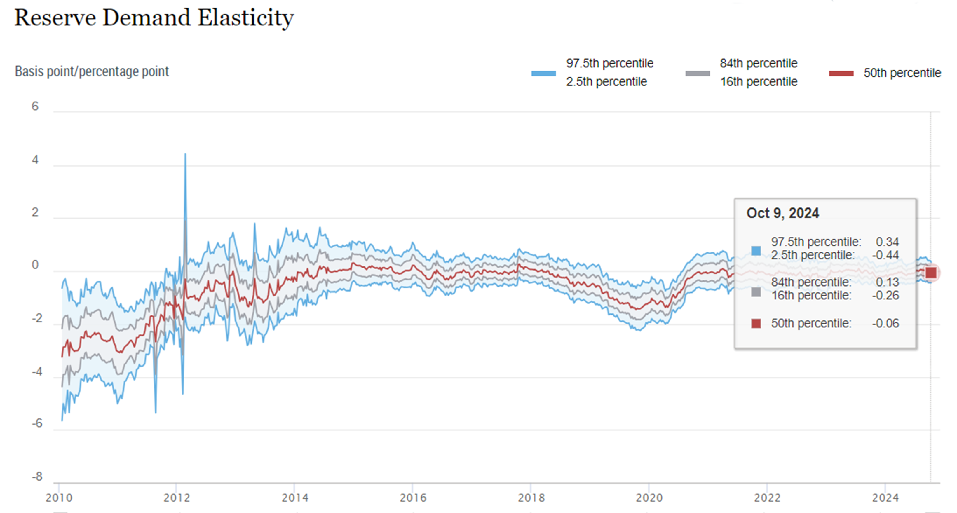
The chart below, taken as a screenshot from the new interactive RDE webpage, shows our real-time estimate of the RDE from January 2010 through October 9, 2024. The RDE was significantly negative in 2010-11 but then became indistinguishable from zero throughout 2012-17 as a result of the large amounts of reserves injected into the banking system by the Federal Reserve in response to the Global Financial Crisis. During the Federal Reserve QT of 2018-19, the RDE returned to be significantly negative at the 68 percent confidence level in August 2018 and at the 95 percent confidence level in March 2019—twelve to six months in advance of the money market turmoil of September 2019. After that episode, the RDE started to move back towards zero, as the Federal Reserve injected liquidity in the banking system to maintain control of short-term rates; since mid-2020, as the Federal Reserve used quantitative easing (QE) in response to the COVID-19 crisis, the RDE has been indistinguishable from zero. Our most recent estimates suggest that, although reserves have declined by over $1 trillion since their peak of $4.2 trillion in November 2021, they remain abundant.

Importantly, today we are launching Reserve Demand Elasticity as a standalone product, with new readings to be published each month on the New York Fed’s public website. The Reserve Demand Elasticity webpage offers the historical and latest estimates of the RDE, as well as information on the underlying data, methodology, and interpretation. The goal of this product is to equip the public with a novel tool that can help in monitoring the ampleness of reserves in the U.S. banking system and stimulate further analysis in this important area.

Gara Afonso is the head of Banking Studies in the Federal Reserve Bank of New York’s Research and Statistics Group.
Domenico Giannone is an assistant director at the International Monetary Fund and an affiliate professor at the University of Washington.

Gabriele La Spada is a financial research advisor in Money and Payments Studies in the Federal Reserve Bank of New York’s Research and Statistics Group.

John C. Williams is the president and chief executive officer of the Federal Reserve Bank of New York.
How to cite this post:
Gara Afonso, Domenico Giannone, Gabriele La Spada, and John C. Williams, “Tracking Reserve Ampleness in Real Time Using Reserve Demand Elasticity,” Federal Reserve Bank of New York Liberty Street Economics, October 17, 2024, https://libertystreeteconomics.newyorkfed.org/2024/10/tracking-reserve-ampleness-in-real-time-using-reserve-demand-elasticity/
BibTeX: View |


 RSS Feed
 Follow Liberty Street Economics
Very interesting topic. I wonder whether if the decline in the volume of Fed funds trading from the pre-ample reserve regime (October 2008) as well as a significantly lower volume of participants causing the overall volume transactions to fall from roundly $250 bln to only about $50bln. It looks to me on the sell side of the market is dominated by the FHLBs, and the Buy side dominated by a relatively small number of foreign banks, not subjected the new (I think 2011) changes in FDIC insurance premiums have change out understanding of the market for Fed funds….As for the September 19, 2019 event, I think the best explanation is that of Copeland and Duffey. Such raises questions as to whether we should placed greater emphasis on the RP rate relative to the funds market