The Macro Effects of the Recent Swing in Financial Conditions

Marco Del Negro, Marc Giannoni, and Micah Smith

Credit conditions tightened considerably in the second half of 2015 and U.S. growth slowed. We estimate the extent to which tighter credit conditions last year were responsible for the slowdown using the FRBNY DSGE model. We find that growth would have slowed substantially more had the Federal Reserve not delayed liftoff in the federal funds rate.

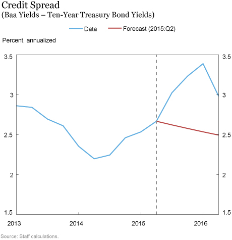
The chart below shows the evolution of credit conditions, as measured by the spread between Baa yields and ten-year Treasury bond yields. One can see that spreads rose considerably from 2015:Q2 to 2016:Q1. This increase was largely unexpected. For instance, the FRBNY DSGE model was forecasting a modest decrease over the coming year as of 2015:Q2 (see the red line). The June 1, 2015, Blue Chip Financial Forecasts consensus was projecting essentially the same decline in spreads.

Increases in credit spreads tend to be associated with subsequent slowdowns in economic activity, with the Great Recession being a salient example. In part, such increases reflect investors’ concerns about future economic conditions, changes in firms’ leverage, heightened worries about borrowers’ default, and so on. However, as Simon Gilchrist and Egon Zakrajšek and others have shown in their research, such increases in credit spreads often cause an economic slowdown. A natural question is then: Did the rise in credit spreads reflect deteriorating economic conditions or did the causality run the other way around in this episode?

To answer this question, we need an economic model that can disentangle the various channels at work. We use the FRBNY DSGE model, which is a very stylized representation of reality that formalizes key interactions among critical economic actors such as households, firms, the financial sector, and the government. The model is then estimated using Bayesian methods, combining prior information about parameters with important macroeconomic data.

The model attributes most of the increase in spreads from 2015:Q3 to 2016:Q1 to unexpected disturbances—which we will refer to as “financial shocks.” These shocks reflect developments that are not fully captured by the model. In late 2015, these developments include a downward revision in the foreign outlook and the deteriorating creditworthiness of the U.S. energy sector owing to the drop in energy prices.

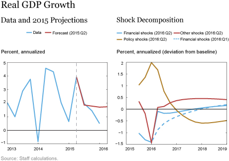
How restrictive, then, has this rise in credit spreads been on the U.S. economy? The left panel in the next chart shows actual growth, from 2013:Q1 to 2016:Q1, in blue. After peaking at 3.9 percent (annual rate) in 2015:Q2, GDP growth slowed markedly for the subsequent three quarters, reaching a paltry 0.5 percent in 2016:Q1. Part of the slowdown was anticipated as of mid-2015: The red line, which indicates the 2015:Q2 forecast, shows that growth was expected to return to just below 2 percent. It just ended up being significantly lower.

The right panel attributes the forecast “miss”—the difference between the blue and the red lines in the left panel—to the various sources of disturbance in the model. Focusing on the effects on growth of the tightening in credit conditions, the blue line in the right panel captures the contribution of the financial shocks that we discussed earlier. These shocks, which are behind the rise in credit spreads, subtracted more than a percentage point from growth (annualized) in each of 2015:Q3, 2015:Q4, and 2016:Q1.

Financial conditions loosened after February 2016, bringing credit spreads back down sharply. Thanks to this reversal in credit spreads, the restrictive effect on GDP growth in the current quarter (2016:Q2) is expected to be much more modest than it would otherwise have been. Had the credit spread reverted to its normal level at its typical pace from February on, it would likely have subtracted another half a percentage point from GDP growth for the rest of 2016, according to the model (see the blue dashed line).

The right panel of the chart above also shows that the tightening in financial condition is not solely responsible for the recent slowdown in GDP growth. Indeed, as indicated by the red line, other shocks subtracted almost 1.5 percentage points from output growth in 2016:Q1. (These shocks reflect various temporary factors, whose effects vanish after 2016:Q1.)

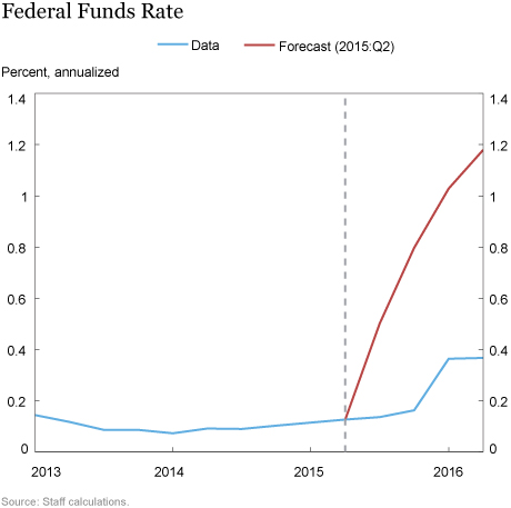
Why did GDP growth not fall by more, then, with such a powerful combination of adverse shocks? According to the model, the answer lies in large part with monetary policy. Recall that as of 2015:Q2, the federal funds rate was expected to rise. For instance, in the March and June 2015 Summary of Economic Projections, the median “dot” for the federal funds rate target was between 0.5 percent and 0.75 percent for the end of 2015. The FRBNY DSGE model was projecting a similar increase, as indicated in the chart below. Both the June 1 and the July 1, 2015, Blue Chip Financial Forecasts projected the policy rate to be 0.5 percent on average in 2015:Q4. However, the FOMC decided to delay liftoff of the federal funds rate. In September 2015, it maintained the target range for the federal funds rate unchanged, citing that “recent global economic and financial developments may restrain economic activity somewhat and are likely to put further downward pressure on inflation in the near term.” The federal funds rate has remained considerably lower than had been forecast in the spring of 2015.

The model suggests that by maintaining the federal funds rate lower, the FOMC managed to substantially offset the effect of tightening financial conditions on the economy. As financial markets revised downward their expectations of interest rate renormalization, the rate at which firms and households could borrow remained low in spite of the increase in spreads. The gold line in the “Shock Decomposition” panel above suggests that the lower federal funds rate path managed to boost GDP growth by more than 1 percentage point for several quarters, essentially offsetting the negative effect of the tightening in financial conditions. In addition, FOMC communication early in 2016 was likely an important factor in the renormalization of financial conditions, although this is not well captured by the model.

In conclusion, the tightening in financial conditions reflected in the rapid rise in credit spreads from 2015:Q3 to 2016:Q1 caused a significant slowdown in growth, according to the FRBNY DSGE model. By delaying the federal funds rate liftoff, the FOMC managed to offset part of these adverse shocks. It is important to remember, however, that our analysis relies on a model that is necessarily a stylized representation of reality. As such, model implications need to be taken with caution.

Disclaimer

The views expressed in this post are those of the authors and do not necessarily reflect the position of the Federal Reserve Bank of New York or the Federal Reserve System. Any errors or omissions are the responsibility of the authors.

---

Marco Del Negro is an assistant vice president in the Federal Reserve Bank of New York’s Research and Statistics Group.

Marc Giannoni is an assistant vice president in the Group.

Micah Smith is a senior research analyst in the Group.

How to cite this blog post:

Marco Del Negro, Marc Giannoni, and Micah Smith, “The Macro Effects of the Recent Swing in Financial Conditions,” Federal Reserve Bank of New York Liberty Street Economics (blog), May 25, 2016, http://libertystreeteconomics.newyorkfed.org/2016/05/the-macro-effects-of-the-recent-swing-in-financial-conditions.html.