


In a 2021 Liberty Street Economics post, we documented the “overnight drift”—a large, persistent return to holding U.S. equity futures in the narrow window between 2:00 and 3:00 a.m. Eastern time, when European equity markets open. Five additional years of data later, that pattern appears to have faded: the 2:00–3:00 window that previously generated roughly 3.7 percent per annum has averaged close to zero since 2021. In this post, we revisit the overnight drift in light of the post-publication sample and use our inventory-risk framework to ask which of three observable channels—the dispersion of closing order imbalances, the level of return variance, or the risk-bearing capacity of liquidity providers—accounts for the change.
The Overnight Drift in One Equation
In our earlier work, we argued that the overnight drift is compensation earned by liquidity providers (LPs)—the participants who post resting limit orders and absorb the residual buy or sell pressure at the end of the U.S. trading day. When institutional flows tilt heavily to one side in the final hour of trading, LPs step in as buyers of last resort and carry the resulting inventory overnight. That inventory is risky: overnight markets are thin, prices can move against the LPs before they can offload, and internal risk limits tighten when volatility is high. To absorb the imbalance at all, LPs demand a discount at the close. As overseas buyers arrive a few hours later—most notably at the Frankfurt and London open—prices rebound, and the LPs earn back their discount. Because overnight markets are thin, even modest incoming order flow moves prices substantially, amplifying the rebound. That rebound is the overnight drift.
As we derive in our paper, in equilibrium, the expected overnight return is the product of three factors:
E[RON] = (dollar order imbalance)t × (return variance)t ×
(risk-bearing capacity)−1.
Each factor is observable: closing order imbalances (Channel 1), return variance (Channel 2), and LPs’ risk-bearing capacity (Channel 3). The drift fades if any one of the three collapses.
Has the Drift Faded in the Post-Publication Sample?
The chart below reproduces the signature pattern over the 1998–2020 sample: a sharp acceleration in cumulative returns between 2:00 and 3:00 a.m. Eastern time, around the European open.
Returns Were Large and Positive Around the European Open from 1998 to 2020
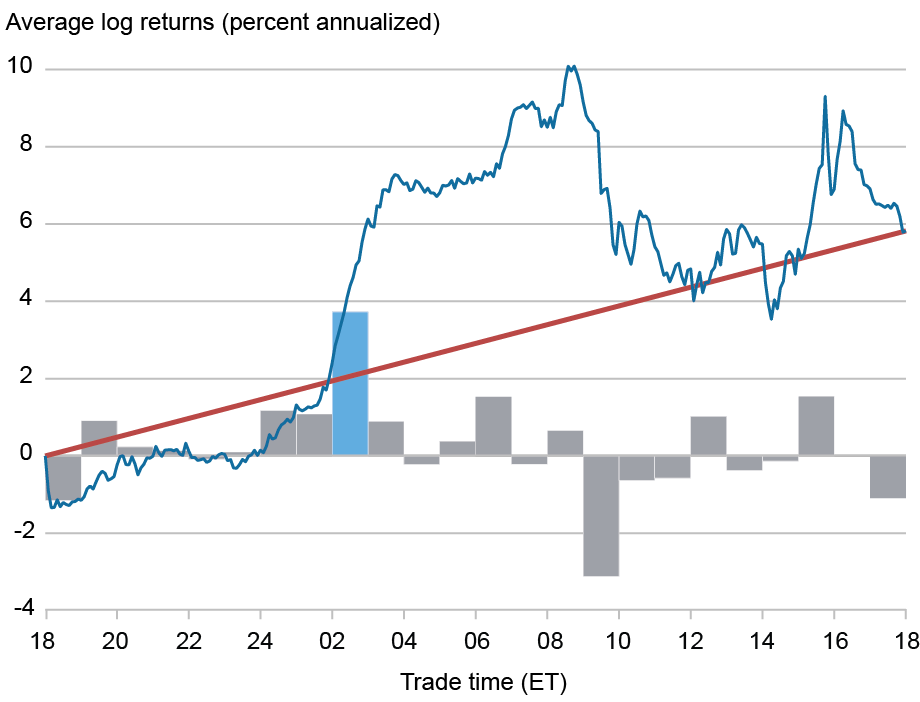
Notes: Sample: S&P 500 E-mini futures, 1998–2020 (5,691 trading days). The bars are average annualized hourly log returns across all trading days in the sample; the solid blue line is the average cumulative 5-minute log return over the trading day. The CME trading day starts at 18:00 ET, so the horizontal axis runs from close to close (18:00 to 18:00). Times are U.S. Eastern. The equation calculating the overnight return is derived in Boyarchenko, Larsen, and Whelan, “The Overnight Drift,” The Review of Financial Studies, Vol. 36, Issue 9, September 2023, Pages 3502–47.
The next chart repeats the exercise for January 2021 through December 2025. The 2:00–3:00 window—previously responsible for more than 60 percent of the contract’s 5.9 percent annualized close-to-close return—is flat. The same pattern holds in the E-mini Nasdaq-100 (NQ) and E-mini Dow Jones (YM) contracts.
But Returns Have Been Flat at the European Open in the 2021-25 Period
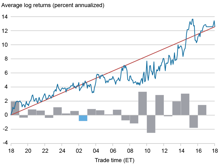
Notes: Sample: S&P 500 E-mini futures, January 2021–December 2025 (1,245 trading days). The bars are average annualized hourly log returns across all trading days in the sample; the solid blue line is the average cumulative 5-minute log return over the trading day. The CME trading day starts at 18:00 ET, so the horizontal axis runs from close to close (18:00 to 18:00). Times are U.S. Eastern.
An episode from an asset management company is illustrative. In June 2022, NightShares launched two ETFs—NSPY and NIWM—designed to capture overnight equity returns by going on long index futures at the U.S. close and selling at the U.S. open; the prospectus cited our inventory-risk mechanism. Both funds were closed fourteen months later, consistent with the weakened pattern over this sample (though ETF-specific costs likely also contributed).
Why Has Overnight Drift Declined?
We now examine how the three channels that lead to the overnight drift—the dispersion of closing order imbalances, the level of return variance, and the risk-bearing capacity of liquidity providers—have evolved since 2020.
The first channel is the magnitude of end-of-day order imbalance. Following our paper, we measure relative signed volume (RSV) during the final hour of U.S. trading (15:15–16:15 ET). RSV is the net buyer-initiated share of last-hour volume, bounded between −1 and +1; it is large and negative on heavy sell-off closes and near zero on balanced days.
The chart below plots the rolling 252-day standard deviation of end-of-day RSV from 1999 through 2025. RSV dispersion trended downward over most of the original sample, and the decline has continued through the post-publication period. Comparing full-sample averages, the standard deviation of end-of-day RSV fell from 6.5 percent to 2.9 percent—a compression of more than half. Extreme closing-imbalance days, which the inventory-risk framework identifies as a source of overnight pricing pressure, have become markedly rarer.
Dispersion of End-of-Day Order Imbalance Has Halved
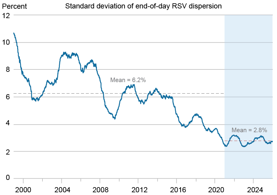
Notes: Rolling 252-day standard deviation of end-of-day relative signed volume (RSV) for the S&P 500 E-mini contract, 1999–2025. RSV is computed over the 15:15–16:15 ET window. Dashed horizontal lines mark period means. The shaded region indicates the post-publication sample (2021–25).
The compression shows up in the predictive relationship between closing imbalances and overnight returns. The next chart sorts days into bins by end-of-day signed volume and traces cumulative next-day returns. In 2007–20 (top panel), large negative closing imbalances are followed by positive overnight returns while large positive imbalances are followed by flat or negative returns—a wide spread concentrated in the overnight window. In 2021–25 (bottom panel), the spread is much narrower, consistent with a weaker predictive link in the post-publication sample.
The Order-Imbalance–Overnight-Return Relationship Has Broken Down
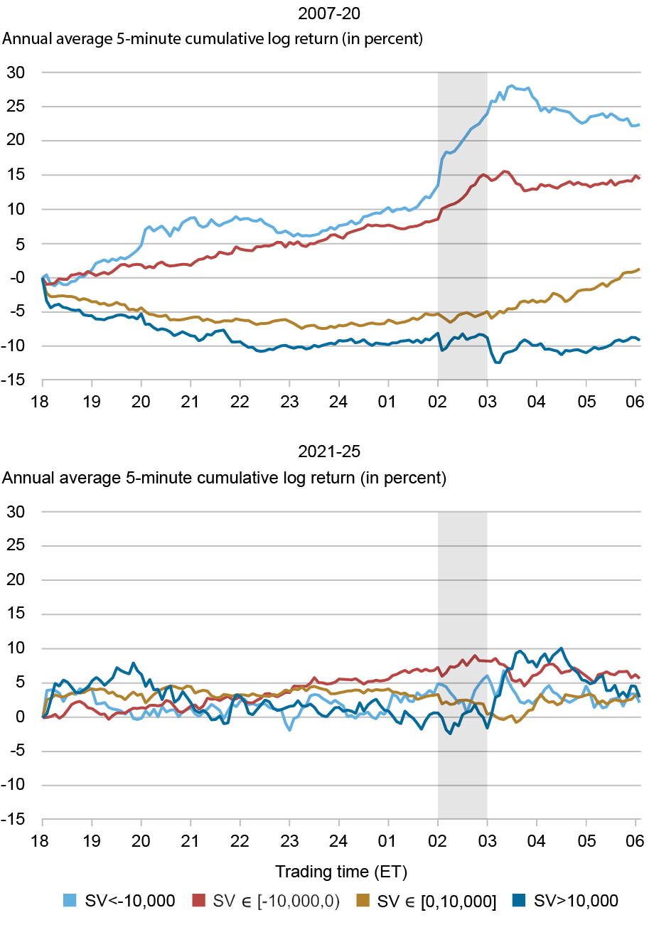
Notes: Cumulative next-day log returns are sorted into four bins by end-of-day signed volume. Shaded regions mark the overnight drift window (2:00–3:00 ET) and the opening reversal (8:30–10:00 ET). Top: 2007–20. Bottom: 2021–25.
Volatility and Liquidity Have Barely Moved
If the compression in closing imbalances accounts for the fade in the drift, our proxies for the other two channels should not themselves have shifted much. Indeed, both appear to be roughly unchanged across samples.
The VIX, a standard proxy for return variance, is little changed: its mean fell only modestly from 20.4 in the original sample to 19.4 in the post-publication period, with median values of 18.6 and 18.2. Overnight liquidity has remained similar in the pre-2020 and post-2020 samples as well—the overnight share of total E-mini volume has edged up only modestly, from 15 percent to 16 percent. On the measures available then, the compression in end-of-day imbalance dispersion is the only input to the pricing equation that has shifted substantially over this period.
What Changed Between the Two Samples?
Our decomposition attributes the bulk of the decline to one input to the pricing equation—the compression in end-of-day imbalance dispersion, while our measures for volatility and overnight liquidity are little changed.
In ongoing work, we find that limit orders posted at the close have become smaller in the post-publication sample, consistent with algorithmic liquidity providers slicing flow more finely and transmitting less residual inventory onto end-of-day counterparties.
Our framework yields a falsifiable prediction: if order-imbalance dispersion widens back toward its pre-2020 range, the overnight drift should reappear in the same 2:00–3:00 window, with the same cross-contract signature. Testing this directly requires a future period of elevated closing-imbalance dispersion, which the current sample does not contain.

Nina Boyarchenko is a financial research advisor in the Federal Reserve Bank of New York’s Research and Statistics Group.
Lars C. Larsen is an assistant professor at Copenhagen Business School.
Paul Whelan is an associate professor at The Chinese University of Hong Kong (CUHK) Business School.
How to cite this post:
Nina Boyarchenko, Lars C. Larsen, and Paul Whelan, “The Disappearing Overnight Drift,” Federal Reserve Bank of New York Liberty Street Economics, July 1, 2026, https://doi.org/10.59576/lse.20260701
BibTeX: View |

Disclaimer
The views expressed in this post are those of the author(s) and do not necessarily reflect the position of the Federal Reserve Bank of New York or the Federal Reserve System. Any errors or omissions are the responsibility of the author(s).
 RSS Feed
 Follow Liberty Street Economics